PSY 652: Research Methods in Psychology I

A Very Brief Intro to Causal Inference

Kimberly L. Henry: kim.henry@colostate.edu

What is Causal Inference?

• Causal inference is about more than finding patterns in data — it’s about understanding what causes what.

• It asks the fundamental question: “If we change one thing, what happens to another?”

• To answer this, we build scientific models that explain relationships between variables using logic and theory.

Why Start with the Scientific Model?

• If our understanding of how things are connected is wrong, no statistical method can fix it.

• Good causal inference requires:

  • Domain knowledge
  • Theoretical understanding
  • Careful thinking about relationships

• Statistical tools can only answer the questions we pose correctly.

Correlation Does Not Imply Causation

An Example: Countries with faster internet speeds (X) have stronger economies (Y). But, correlation is likely spurious because wealthier countries are more likely to invest in advanced infrastructure, including high-speed internet. Economic strength and internet speed are both outcomes of higher national wealth.

But Also, Causation Does Not Imply Correlation

An Example: When cruise control is set on a car, changes in road incline (X) causally affect the engine’s power output (Z) to maintain the set speed (Y). Despite the causal effect of road incline on engine power, the vehicle speed Y remains constant due to the cruise control. Data collected on vehicle speed (Y) and road incline (X) will show no correlation, despite X causing Y. The cruise control is an example of a feedback control mechanism.

Potential Outcomes Framework

Last week, you made a decision to either:

• Read the Module 18 material (\(x_i = 1\))

• Not read the Module 18 material (\(x_i = 0\))

Which of these actions will be better for your comprehension of today’s lecture?

Definition of Variables

• We’ll label the treatment/exposure, reading the material, as \(x_i\).
• We’ll label the outcome, comprehension of the lecture, as \(y_i\).

The Potential Outcomes

We have two potential outcomes in this scenario:

• One represents your comprehension if you read the material: \(y_i(1)\)

• The other represents your comprehension if you didn’t read the material: \(y_i(0)\)

If you read the Module 18 material prior to class:

• We observe \(y_i(1)\)
• The outcome \(y_i(0)\) remains the counterfactual (unobserved)

If you didn’t read the Module 18 material prior to class:

• We observe \(y_i(0)\)
• The outcome \(y_i(1)\) remains the counterfactual (unobserved)

The Individual-Level Causal Effect

• The individual‐level causal effect is: \[y_i(1) - y_i(0)\]

• That is — the difference in your comprehension of the lecture if you read the Module 18 material versus if you didn’t read the material.

• This difference is unknowable!

• This is the fundamental problem of causal inference (Holland, 1986).

Random Assignment to Condition

Let’s imagine that I randomly assign half of you to read the Module 18 material and the other half to not read the material.

• If you’re assigned to read the material, and you read it — then we observe \(y_i(1)\).

• If you’re not assigned to read the material, and you don’t read it — then we observe \(y_i(0)\).

Therefore, we can compute the Average Causal Effect as:

\[ \text{Average Causal Effect (ACE)} = E[y_i(1)] - E[y_i(0)] \]

The Incredible Power of Randomization

Randomization is a tremendously powerful procedure for examining causal effects. However, it’s not always perfect in practice:

• Non-compliance: Participants don’t follow treatment assignment

• Drop-out: Participants fail to provide outcome data

• Unmanipulable causes: Some causes cannot be directly manipulated (e.g., emotional responses)

• Ethical and practical constraints: Randomization might be unethical (e.g., drug use) or unfeasible (e.g., socioeconomic status)

Roadmap: When Perfect Experiments Aren’t Possible

Today we’ll learn about tools for causal inference:

1. Directed Acyclic Graphs (DAGs) — Visual models of causal relationships

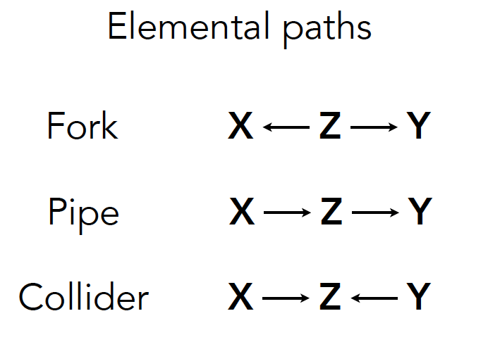
2. Three Key Structures — Forks, Pipes, and Colliders

3. Identification Strategy — How to determine what variables to control for

4. What Can Go Wrong — Why controlling for the wrong variables can bias results

What to Do Absent a Perfectly Executed Experiment?

In these scenarios, it’s helpful to think about the entire causal network underlying the data. Graphical notation can make it easier to understand and analyze these complex relationships.

Directed Acyclic Graphs (DAGS)

DAGS are a powerful and intuitive tool for representing causal relationships.

• Heuristic Models: DAGs are simplified representations of a causal model, focusing on the structure of relationships rather than exact mechanisms or mathematical details.

• Directed: Each arrow shows the direction of influence between two variables. An arrow from X → Y means X is assumed to cause Y (but not the other way around).

• Acyclic: DAGs do not allow loops or cycles—no variable can directly or indirectly cause itself. This ensures clarity in identifying causal pathways.

• Anonymous Influence: DAGs don’t specify how variables influence each other (e.g., linear or nonlinear effects); they only indicate that one variable influences another.

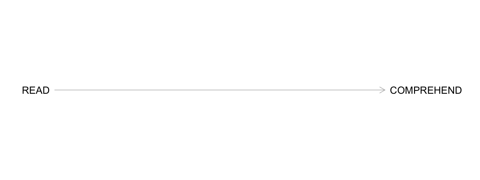
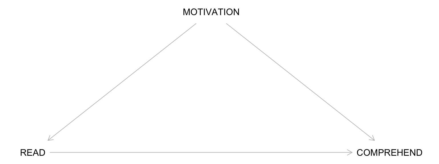
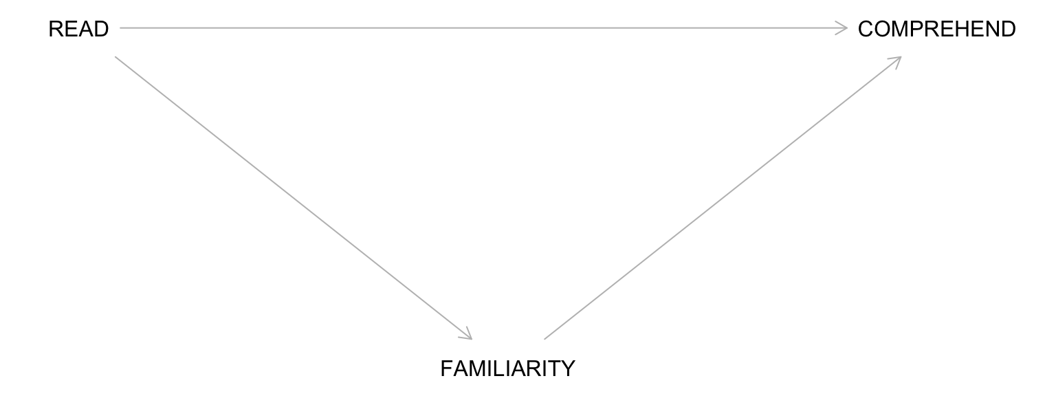
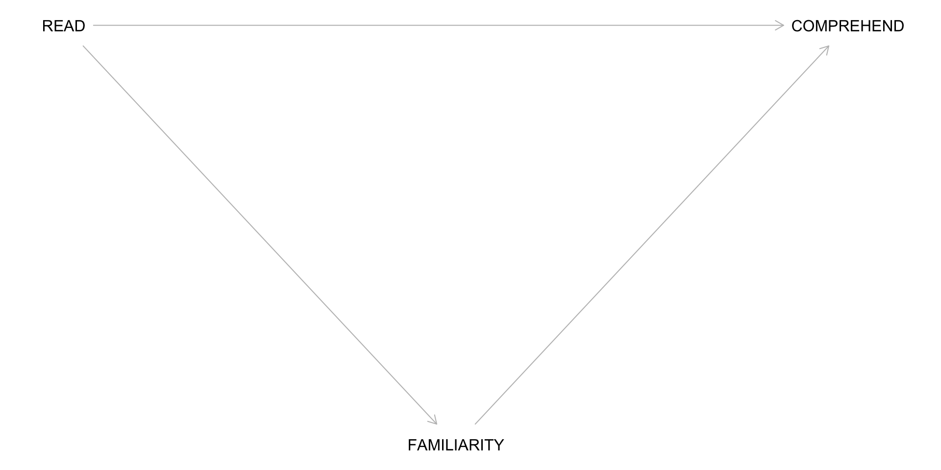
An Example DAG

Start by drawing the exposure (e.g., reading the material) and the outcome (e.g., comprehension of the lecture).

Building a Complete DAG: Step 1

Draw all common causes of X and Y – including measured and unmeasured variables.

• Common causes create confounding
• Omitting them means assuming they don’t exist
• Both observed and unobserved confounders should be represented

Building a Complete DAG: Step 2

As you add new variables, include any common causes of any pair of variables in your DAG.

• This ensures that the DAG accounts for potential bias introduced by shared causes
• Keep building until you’ve represented all confounding relationships

If there are variables through which X affects Y (i.e., mediators):

• Draw arrows from X to the mediator(s)
• Draw arrows from the mediator(s) to Y

Building a Complete DAG: Step 3

Include all selection variables – these represent selection processes that occur as part of the study:

• Drop out
• Death
• Non-compliance
• Sample selection

Critical Assumption

Drawing a DAG requires expert knowledge and must be complete! NOT including an arrow implies an ASSUMPTION that there is NO CAUSAL EFFECT.

Consider an Observational Version of the Study

For the READ to COMPREHENSION example, let’s imagine I simply assessed whether students chose to read the material:

Will the difference in comprehension between those who chose to read vs. not read represent an average causal effect?

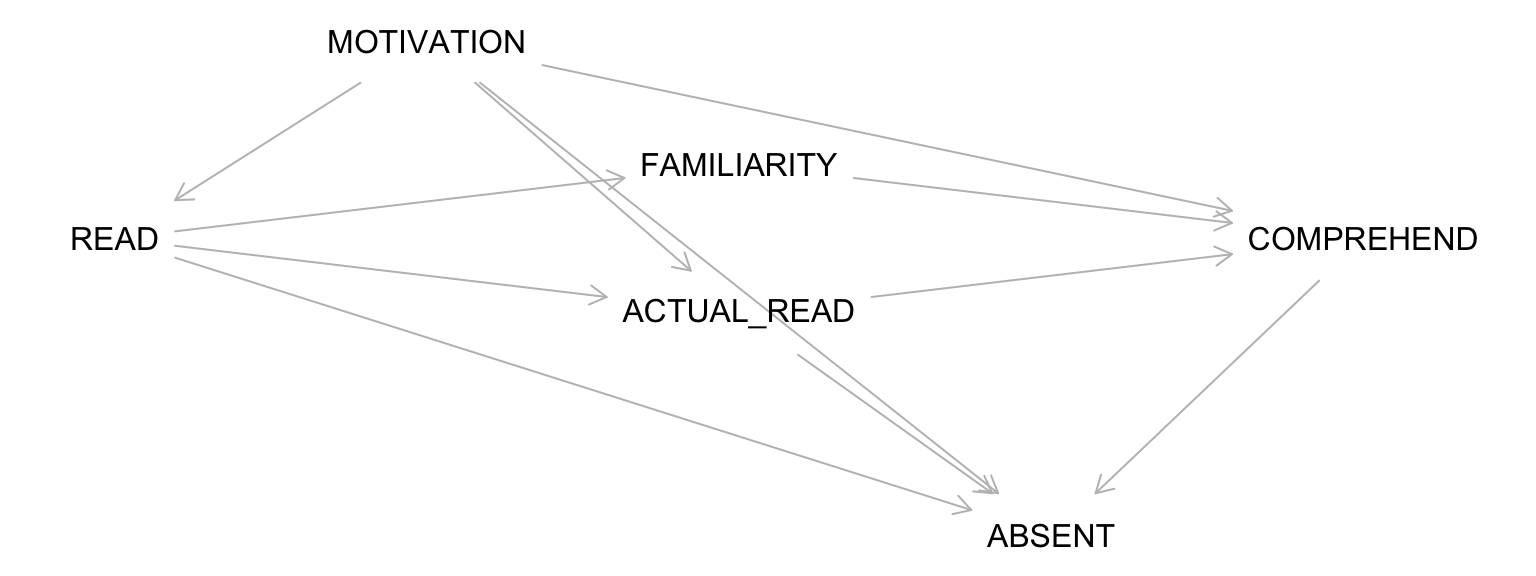
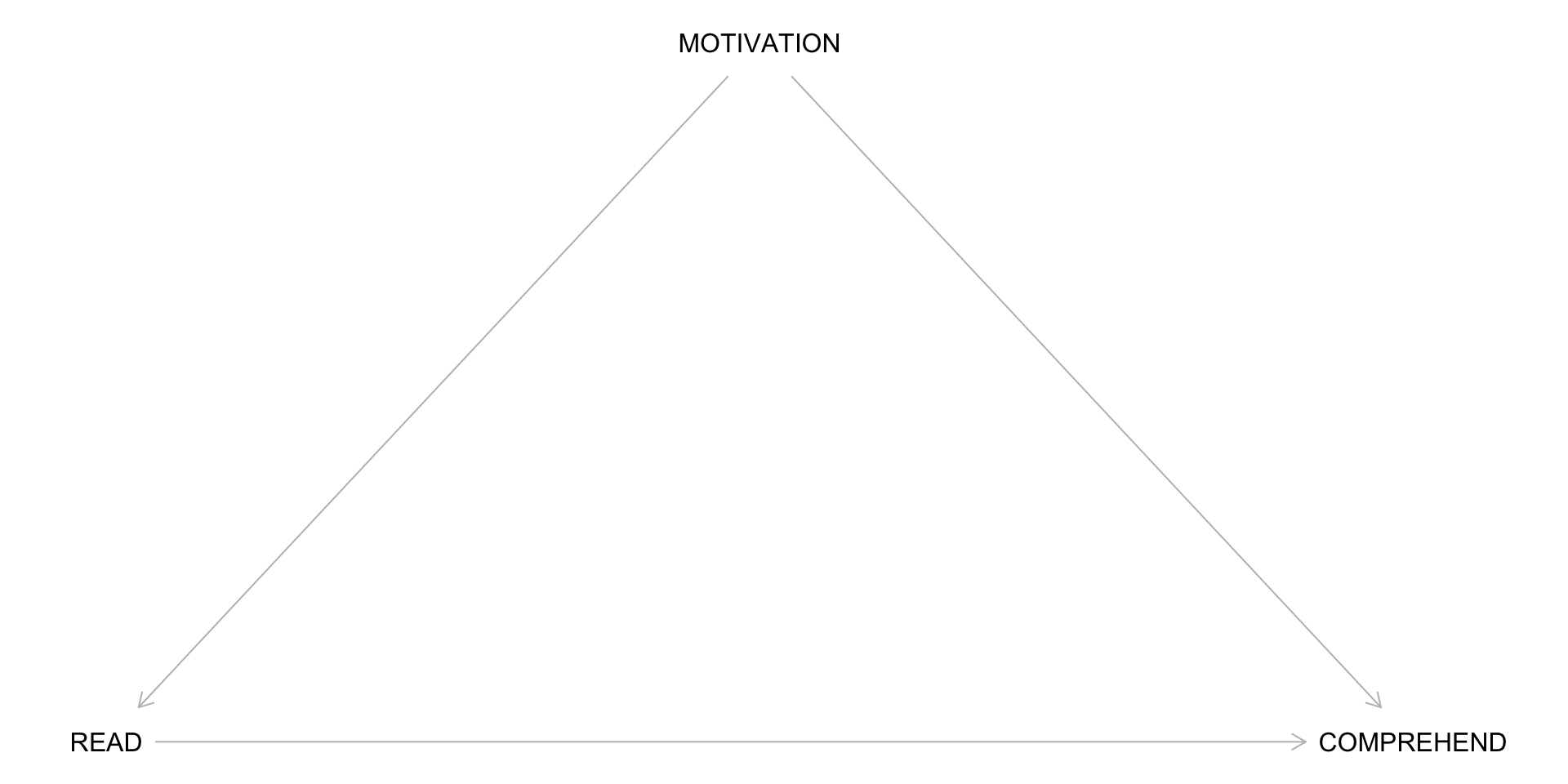
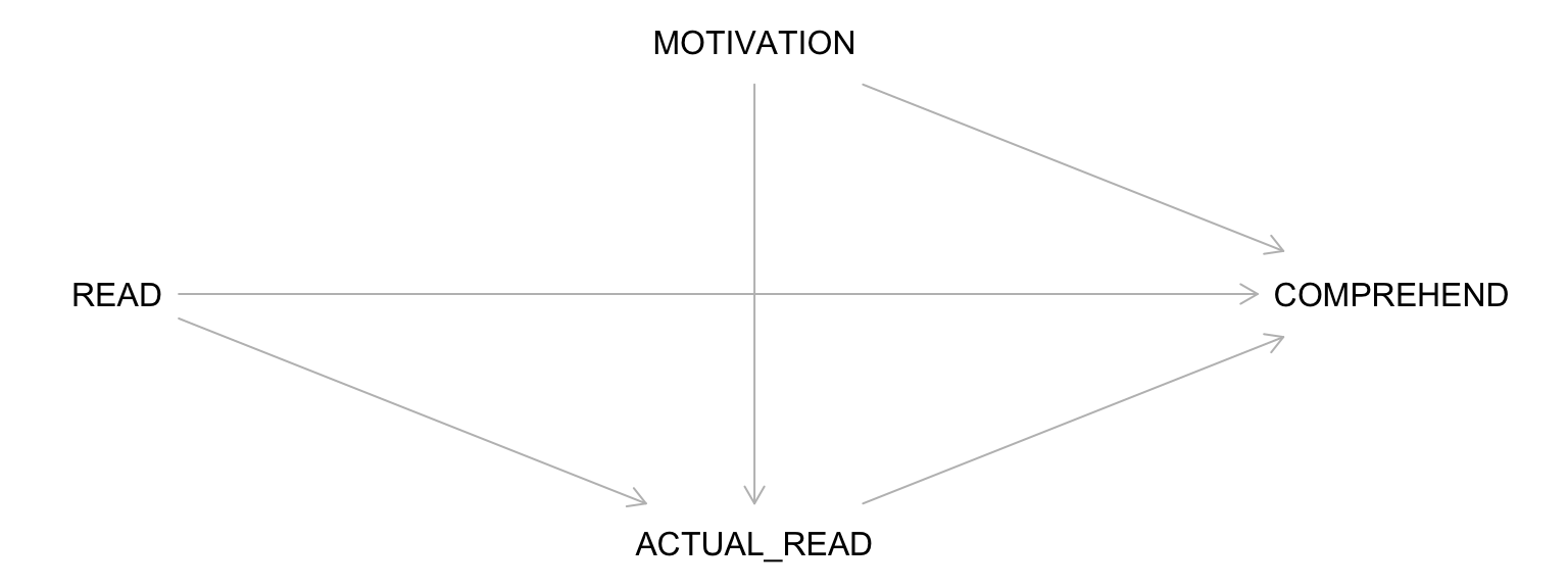
A DAG for the Observational Study

Understanding Paths in DAGs

• Path: A sequence of arrows between two variables in a DAG, not passing through any variable more than once. The direction of the arrows is irrelevant when defining a path.

  • Causal Paths: All arrows point in the same direction, from cause (X) to effect (Y). This path represents a direct or indirect causal relationship.

  • Non-Causal Paths: Include at least one arrow that points toward X (or away from Y). These paths may introduce confounding or other non-causal associations.

Visual Guide

Causal: X → Z → Y (all arrows forward)

Non-causal: X ← Z → Y (includes backward arrow)

Identify the Paths Connecting X to Y

1. READ → COMPREHEND (causal path)

2. READ ← MOTIVATION → COMPREHEND (non-causal path / back-door path)

Block the Back Door Path(s)

• A back-door path connects the exposure (X) to the outcome (Y) through a common cause — also called a confounder.

• Conditioning on the confounder (e.g., adjusting for MOTIVATION) blocks the back door path.

• This breaks the spurious connection and isolates the causal effect.

Three Key Structures in DAGs

The Fork

A Fork is a Confounder Scenario

READ ← MOTIVATION → COMPREHEND

Key Property: The fork creates a non-causal association between READ and COMPREHEND through their common cause, MOTIVATION.

Generate Data

What do you Predict?

Before running the code, make a prediction:

What will happen to the relationship between X and Y when we:

1. Don’t control for Z?

2. Control for Z?

Graph the Data

Fit the Models

Take Home Message

What we observed:

• Without controlling for Z: We see a spurious association between X and Y
• After controlling for Z: The association disappears, revealing no true causal effect

Lesson: When you have a fork (confounder), you must control for it to get an unbiased estimate of the causal effect.

# The correct model:
lm(COMPREHEND ~ READ + MOTIVATION, data = df)

Contrast: A Properly Executed Experiment

READ → COMPREHEND (causal path only)

Notice: Random assignment breaks the arrow from MOTIVATION to READ!

Simulate an Experiment

Plot Data from Simulated Experiment

Fit Models from a Simulated Experiment

The Pipe

The Pipe is a Mediator Scenario

READ → FAMILIARITY → COMPREHEND

Key Property: The pipe represents a causal pathway through which X affects Y.

Familiarity as the mechanism

Reading the material causes familiarity with it, which in turn promotes better comprehension during the lecture.

Identify the Paths Connecting X to Y

1. READ → COMPREHEND (causal path)

2. READ → FAMILIARITY → COMPREHEND (causal path – pipe)

Proper Handling of Pipes

• If You Want the Total Effect:

  • Do not adjust for the mediator

  • Simply estimate the overall effect of READ → COMPREHEND

  • Otherwise, you will “explain away” part of the effect of interest

• If You Want the Direct Effect:

  • You can adjust for the mediator, but interpretation of the exposure takes extra care

  • This is the domain of mediation analysis

Generate Data

What do you Predict?

Before running the code, make a prediction:

What will happen to the coefficient on X when we:

1. Don’t control for Z (the mediator)?

2. Control for Z?

Graph the Data

Fit the Models

Interpreting the Pipe Simulation

What we observed:

• Without controlling for Z: We see the total causal effect of X on Y (through Z)
• After controlling for Z: The effect of X disappears because Z is the mechanism

Lesson: When you have a pipe (mediator), controlling for it blocks the causal pathway you’re interested in. Don’t control for mediators if you want the total effect!

# The correct model for the total effect of READ:
lm(COMPREHEND ~ READ, data = df)

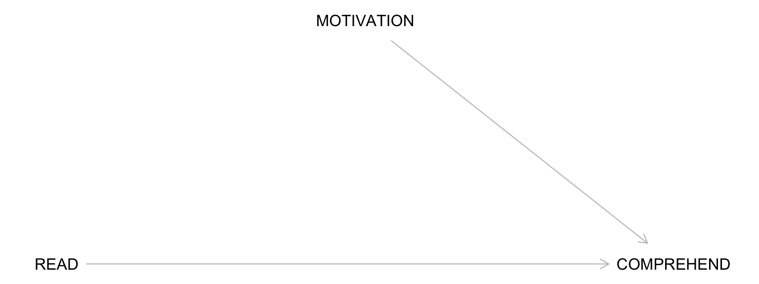
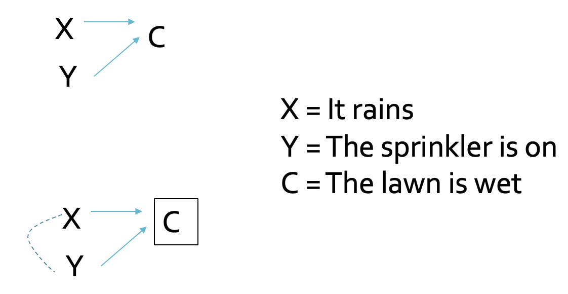
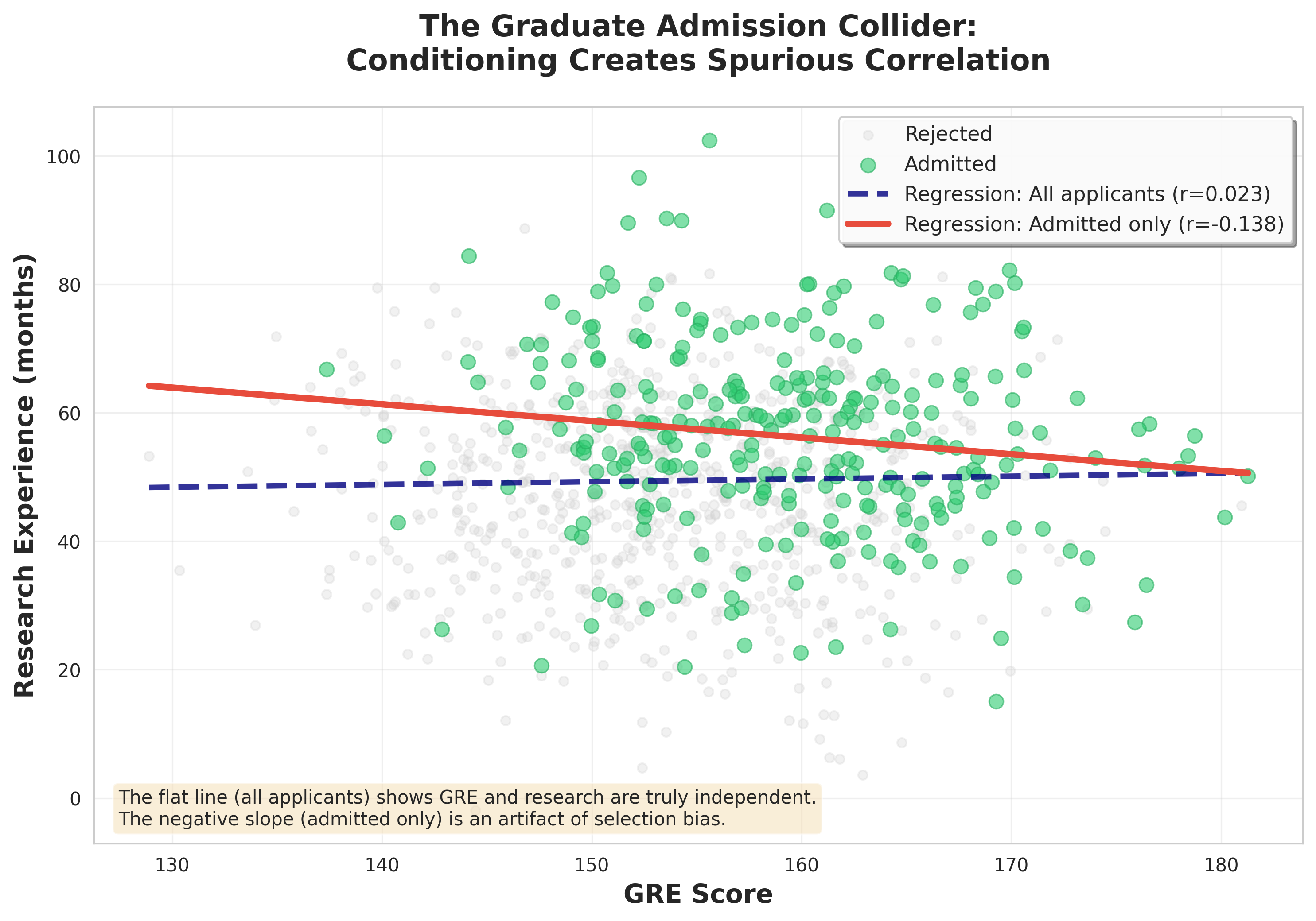
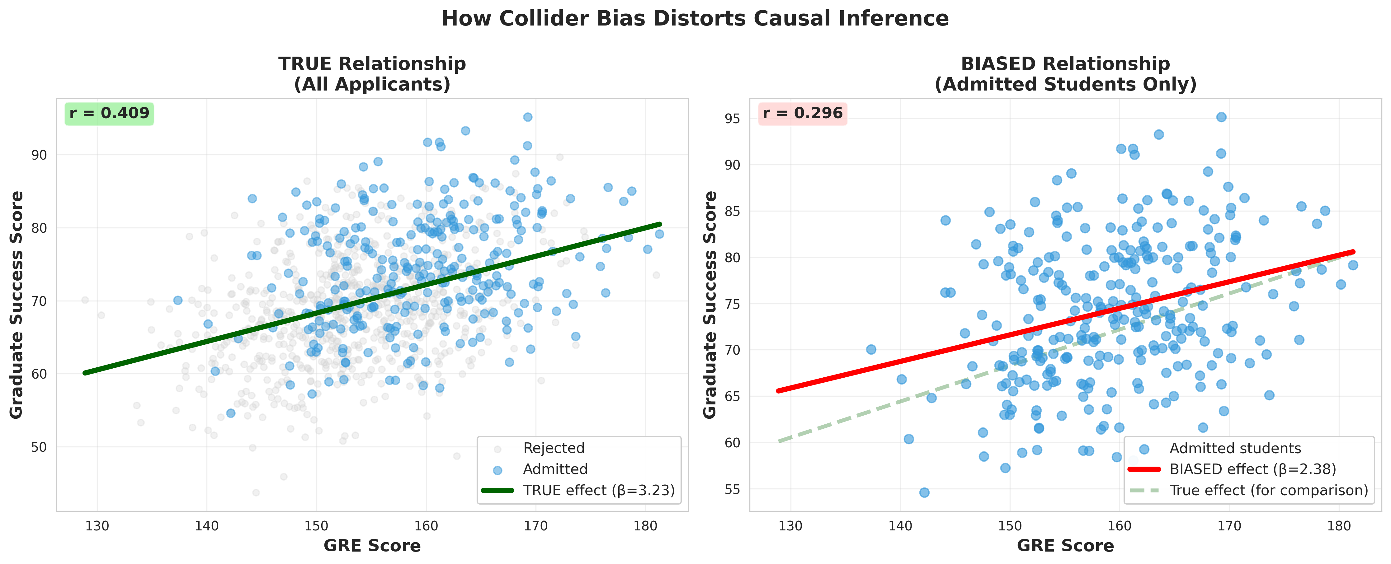
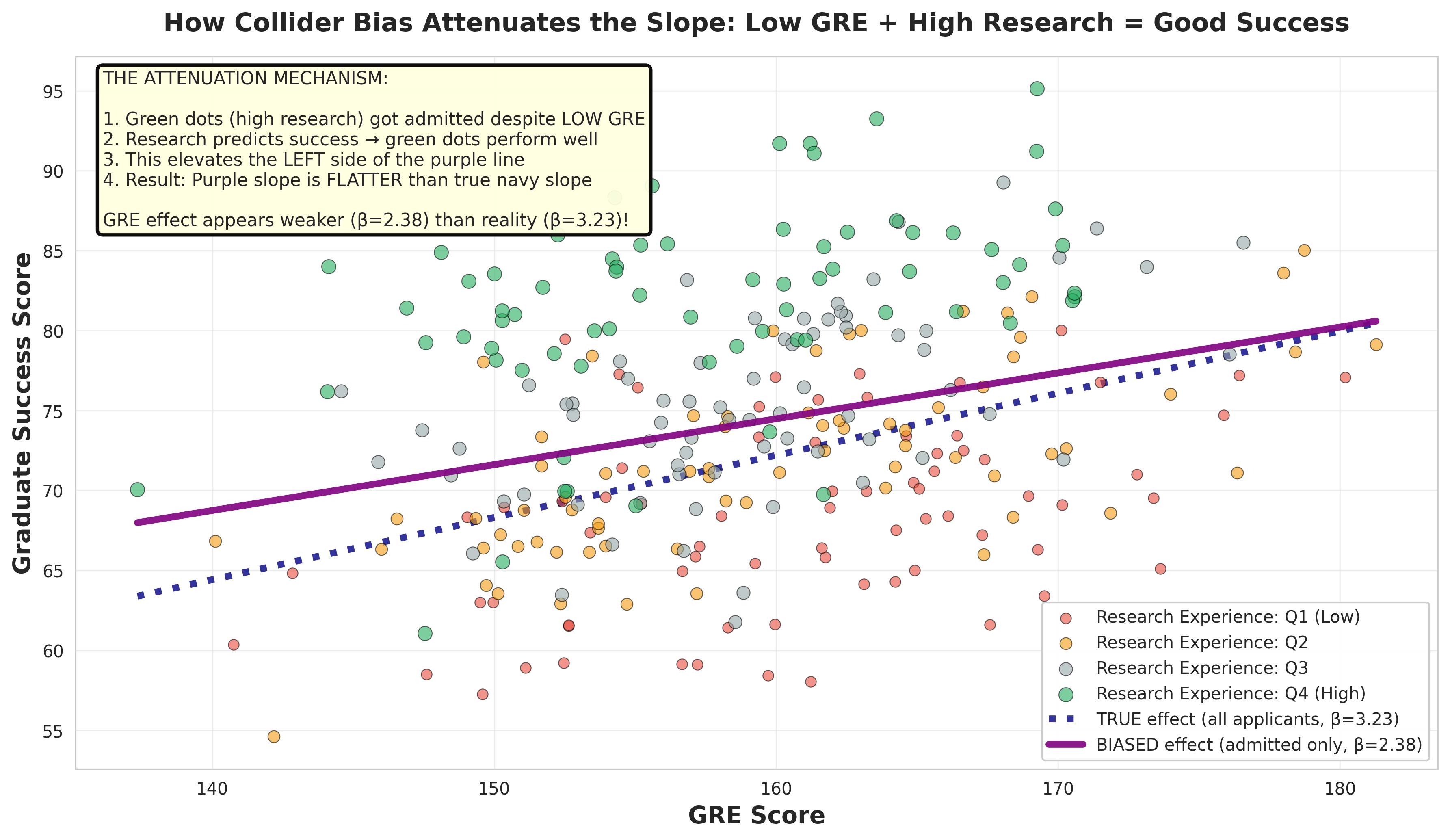
The Collider

Colliders are a Scary Scenario

Key Property: A collider is caused by two or more variables. By default, collider paths are blocked.

An Intuitive Example of a Collider

Question: Are “Rain” and “Sprinkler On” correlated?

Intuition: Conditioning on a Collider

Scenario 1 - Not conditioning on “Lawn Wet”:

• Rain and Sprinkler are independent
• No correlation expected

Scenario 2 - Conditioning on “Lawn Wet = Yes”:

• If we know the lawn is wet AND it didn’t rain…
• Then the sprinkler must have been on!
• This creates a spurious negative correlation

Lawn Simulation: Make a Prediction

Before running the simulation, predict:

1. What will be the correlation between Rain and Sprinkler in the full data?
2. What will be the correlation when we condition on Lawn Wet?

Lawn Simulation Results

Proper Handling of Colliders

• By default, collider paths are blocked, meaning they do not create a spurious association between the exposure and the outcome.

• But beware: If you condition on a collider, you will open a back door path and create a spurious association.

Critical Rule

Never condition a collider unless you have a very good reason and understand the implications!

Collider Example: Bias When Selecting the Sample

Extending to an Outcome

The Mechanism

Collider Example: Non-compliance

The Mechanism

Non-Compliance as a Collider in the Read Example

READ -> COMPREHEND (causal path)
READ -> ACTUAL_READ -> COMPREHEND (causal path – pipe)
READ → ACTUAL_READ ← MOTIVATION → COMPREHEND (collider)

What Model Should be Fit for the Experiment?

# The correct model:
lm(COMPREHEND ~ READ, data = df)

# DO NOT include ACTUAL_READ in the model!

Why?

• By conditioning on ACTUAL_READ, you open a non-causal path between READ and MOTIVATION that would otherwise remain blocked (collider bias)

• This creates a spurious association between READ and COMPREHEND, undermining the causal interpretation

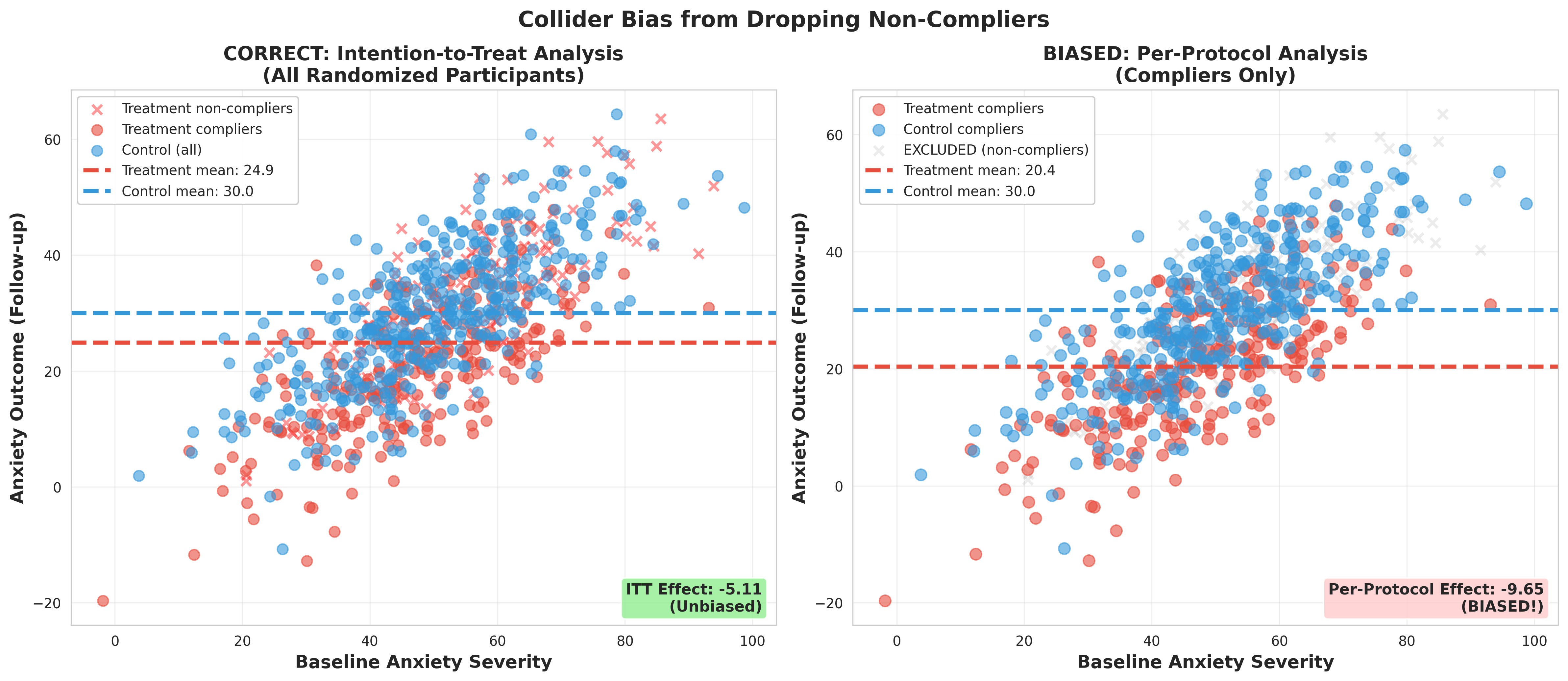
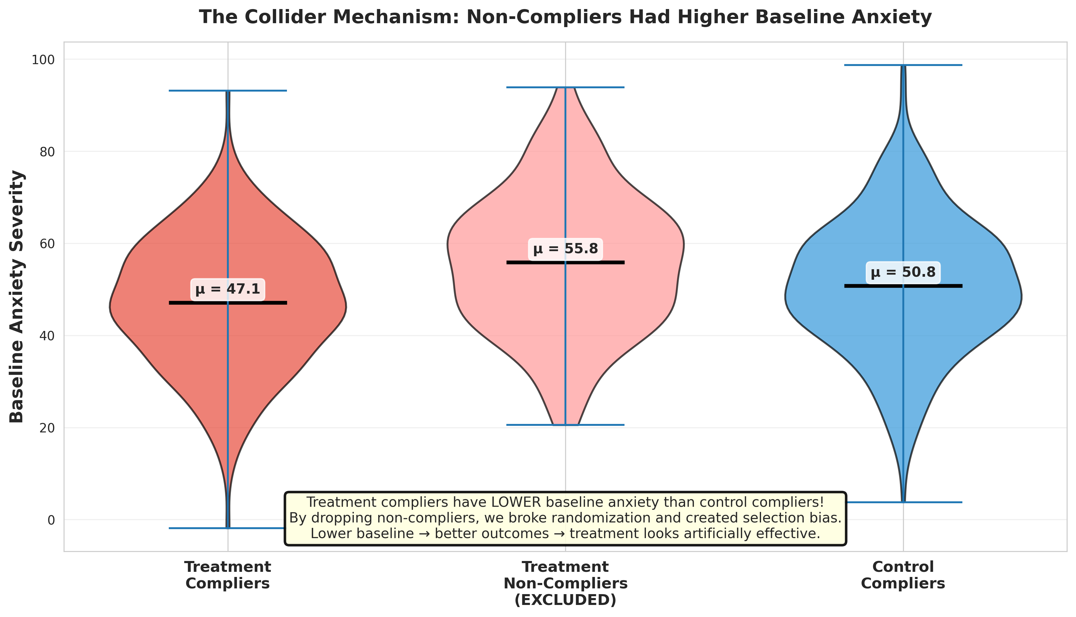
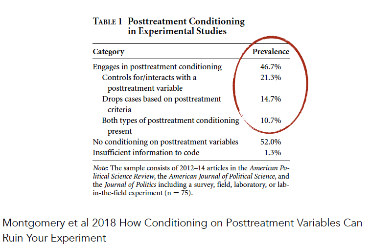
• Revel in the beauty of your experiment, and don’t include any post-treatment variables! Don’t drop non-compliers and don’t control for non-compliance in a model.

Take Home Message for Experiments

Many researchers make this mistake! Understanding DAG structures helps you avoid it.

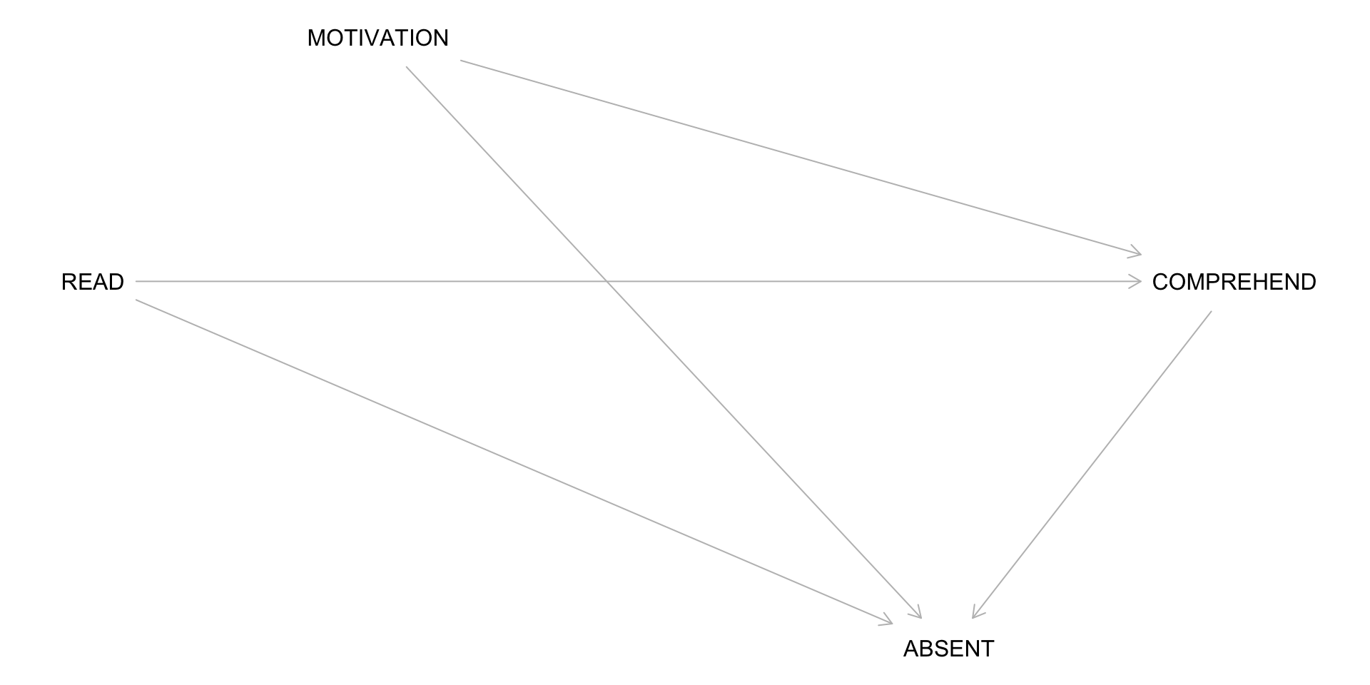
Another Common Collider: Dropout

In field experiments, participants often drop out before outcome measurement.

Let’s add ABSENT to our DAG:

READ -> COMPREHEND (causal path)
READ -> ABSENT <- COMPREHEND (collider)
READ -> ABSENT <- MOTIVATION -> COMPREHEND (collider)

Dropout is a Collider

Being ABSENT may be caused by:

• Treatment assignment (READ)
• The (potential) outcome itself (COMPREHEND)
• Motivation (MOTIVATION)

When students are absent, we don’t observe their COMPREHEND score.

If we analyze only students with observed outcomes:

• We are implicitly conditioning on ABSENT = 0
• This opens back-door paths that were blocked!

The Problem: Listwise Deletion

When you run a standard regression with missing outcomes:

# R automatically drops rows where COMPREHEND is NA
lm(COMPREHEND ~ READ, data = df)

This is equivalent to:

# Filtering to only completers
lm(COMPREHEND ~ READ, data = df |> filter(ABSENT == 0))

You are conditioning on the collider ABSENT, which:

• Opens back-door paths: READ → ABSENT ← MOTIVATION → COMPREHEND and READ -> ABSENT <- COMPREHEND
• Creates selection bias (even in a randomized experiment!)

Solution: Use principled missing data methods (multiple imputation, inverse probability weighting, sensitivity analyses)

Summary of the Three Structures

A Guide for Proceeding

Structure	Default State	What to Do	Why
Fork (X ← Z → Y)	Path is OPEN	Control for Z	Blocks confounding
Pipe (X → Z → Y)	Path is OPEN	Don’t control for Z (for total effect)	Preserves causal pathway
Collider (X → Z ← Y)	Path is BLOCKED	Don’t control for Z	Avoid inducing spurious association

References and Resources

• Holland, P. B. (1986). Statistics and causal inference. Journal of the American Statistical Association.

• McElreath, R. (2020). Statistical Rethinking (2nd ed.). CRC Press.

• Pearl, J., Glymour, M., & Jewell, N. P. (2016). Causal inference in statistics: A primer. Wiley.

• Hernán, M. A., & Robins, J. M. (2020). Causal Inference: What If. CRC Press.

• Dr. Julia Rohrer’s Teaching and Learning Paper: Causal inference for Psychologists who think causal inference isn’t for them. (This slide deck builds on one of her examples)

• DAGitty: http://dagitty.net