PSY 652: Research Methods in Psychology I
Random Sampling for Parameter Estimation
Kimberly L. Henry: kim.henry@colostate.edu
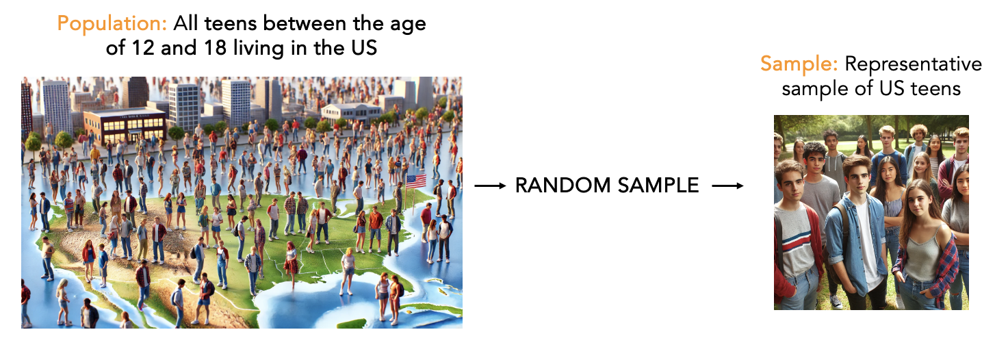
A population and a random sample
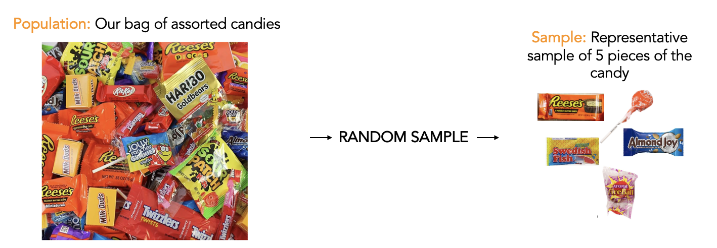
The Great Candy Sampling Experiment 🍬
Our bag of candy analogy
Candy data
Let’s import the candy data population.
The data are stored in an excel file called candy_2025.xlsx — this file has multiple sheets/tabs. Here, we are reading in the sheet/tab labeled population. The read_excel() function from the readxl package is used.
Full data frame of candy population data to peruse
Our Population: 100 Pieces of Candy
Let’s describe the population.
We will define the total weight of the 100 pieces of candy as our population parameter.
Part 1: Student Selections (Convenience Sample)
Import the data
Starting point: the wide data frame
The original data frame has 11 columns:
So for every student, we have 5 pairs: (label_1, weight_1), (label_2, weight_2), …, (label_5, weight_5).
Problem
This “wide” format makes it harder to analyze because the label–weight pairs are spread across columns. We’d like each pair to become its own row, so we end up with just three columns, where each student has five rows of data — one for each piece of selected candy:
- name: student name
- label: the label of the candy
- weight: the weight of the candy
What the code does
The pivot_longer() step takes all of the label and weight columns and reorganizes them into a “long” format. Instead of having 10 columns, we get more rows. This application looks a bit different than previous examples we’ve seen because there are two variable series that we need to pivot (label and weight).
The argument names_to = c(".value", "item"), names_sep = "_" tells R how to split the old column names. For example, “label_3” is split into two parts: “label” and “3”. The special keyword .value means that R should create new columns named label and weight. The item part just keeps track of which number (1–5) the values came from.
After pivoting, each row has three pieces of information: the item number, the label, and the weight. The final data frame is “long” and tidy, and will be easy to work with.
Full data frame of student samples to peruse
Use your sample to predict the total weight
Each of you drew 5 pieces of candy (your sample). Let’s use your sample to estimate the total weight of all 100 pieces.
How to estimate:
Compute your sample mean (average) weight.
Multiply by 100 (because there are 100 candies in the bag).
Average estimated parameter
We can now compute the average parameter estimate (total weight of all candies) across the 20 student samples.
How did we do? Convenience vs. Reality
Did your samples do a good job of predicting the weight of all 100 pieces?
Question: Why do you think most students overestimated? 🤔 What was your Data Generating Process?
Part 2: Simple Random Sampling (SRS)
Let’s try Simple Random Sampling instead
Can random sampling get us closer to the truth?
Let’s draw 20 random samples of size 5.
Comparison: Convenience vs. Random Sampling
Bias = How far off we are, on average
- Formula: Mean of all sample estimates - Population parameter
Percent Error = How far off we are as a percentage
- Formula: (|Bias| / Population parameter) × 100
Population parameter: 2388.9
Key Insight: Random sampling reduces bias! 🎯
Part 3: The Sampling Distribution
What is the sampling distribution?
Now, let’s dig into the concept of a sampling distribution.
The sampling distribution is the distribution of a statistic (like a sample mean, or a sum, or a proportion) calculated from multiple random samples of the same size, taken from the same population.
For example, the estimated weight of all candies based on many, many repeated samples.
Simulate random sampling from the population
Let’s create a sampling distribution using the candy data, we’ll simulate 1000 random samples of size 25 from the “population” (i.e., the 100 pieces of candy). We’ll also do this resampling with replacement.
With replacement means we put each candy back before the next pick, so the bag never changes — every draw has the same chances as the last, and each of our 1000 samples truly comes from the same population, which is exactly what we want for a clean sampling distribution.
Create a histogram of the parameter estimates
The distribution of the parameter estimates across all possible random samples is the sampling distribution.
What are some key properties of the sampling distribution?
Some key properties of the sampling distribution
Centered on the Population Parameter: The sampling distribution tends to cluster around the true population parameter. The mean of the parameter estimates across random samples equals the true parameter (provided samples are sufficiently large).
Variability: The spread of the sampling distribution reflects how much the statistic fluctuates around the population value. The standard deviation of the sampling distribution is called the standard error, and describes how much sample to sample variability we expect.
Normality (Central Limit Theorem): With a sufficiently large sample size, the sampling distribution is approximately normal, regardless of the population’s shape.
Part 4: Effect of Sample Size
Does sample size matter?
Let’s explore how sample size affects our estimates of the parameter (total weight).
We’ll use a custom function called simulate_random_samples().
We’ll move from a histogram to a density graph to display the sampling distribution.
Explore sample size
Please use the function to vary the sample size. See what happens as you change the sample size to:
2, 5, 10, 25, 50
What changes when sample size increases?
Shape: The sampling distribution of the statistic (e.g., looks more normal (thank you, CLT)).
Spread: Estimates cluster more tightly around the truth; the standard error shrinks .
Extremes: Fewer extreme estimates show up.
Why this matters
A (roughly) Normal sampling distribution lets us use the Normal’s built-in cut points to mark what’s typical vs. unlikely (e.g., the middle ~95% ≈ 1.96×SE).
That “probability ruler” is exactly what powers confidence intervals and hypothesis tests.
Bottom line: with random sampling, bigger n makes estimates steadier and more trustworthy.
Two quick cautions:
Random sampling is key—bigger n doesn’t fix bias from convenience samples.
Very skewed/heavy-tailed populations may need larger n before the Normal approximation is good.