Participants imagined being athletes competing in a boulder-sliding game against an opponent named Blorg. The goal was to slide a boulder farther on ice to win a prize.
A Special Boulder
Participants could rent a “special boulder” — a possibly advantageous upgrade expected to improve performance.
The Conditions
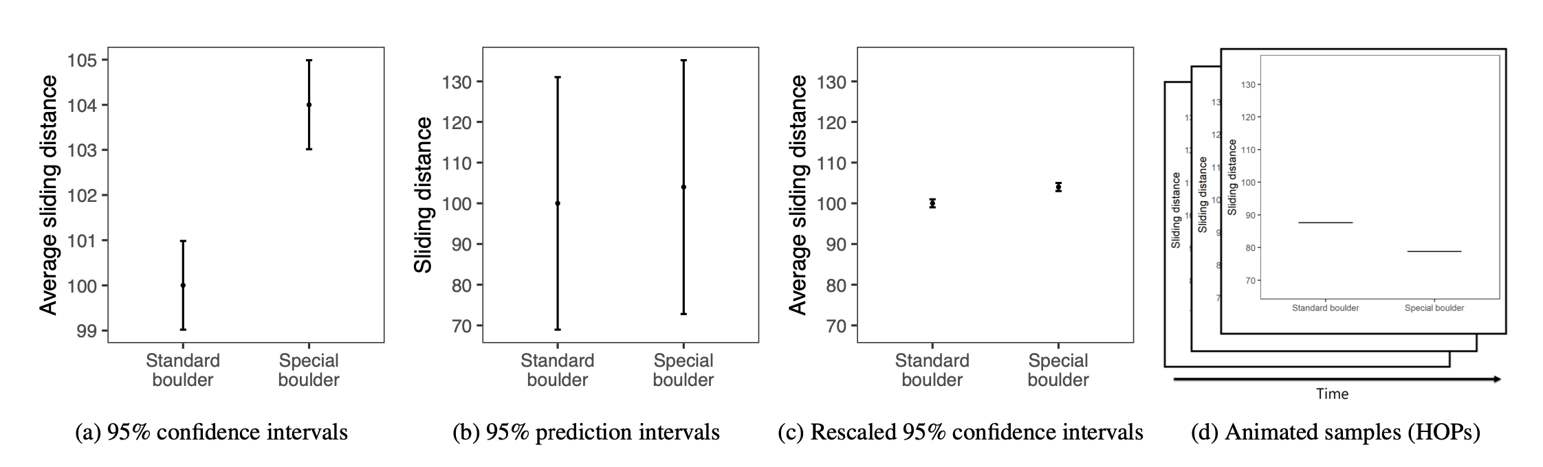
To help decide whether to rent the special boulder, each participant saw one of four uncertainty visualizations summarizing prior results.
The Outcome
After viewing their assigned visualization, participants estimated the probability that using the special boulder would help them win. We’ll refer to this as perceived win probability.
The Data
graph_type: visualization type (CI, PI, CI rescaled, HOPS) — randomly assigned
superiority_special: perceived probability that the special boulder would win (0–1)
Visualize the Data
Our Research Question
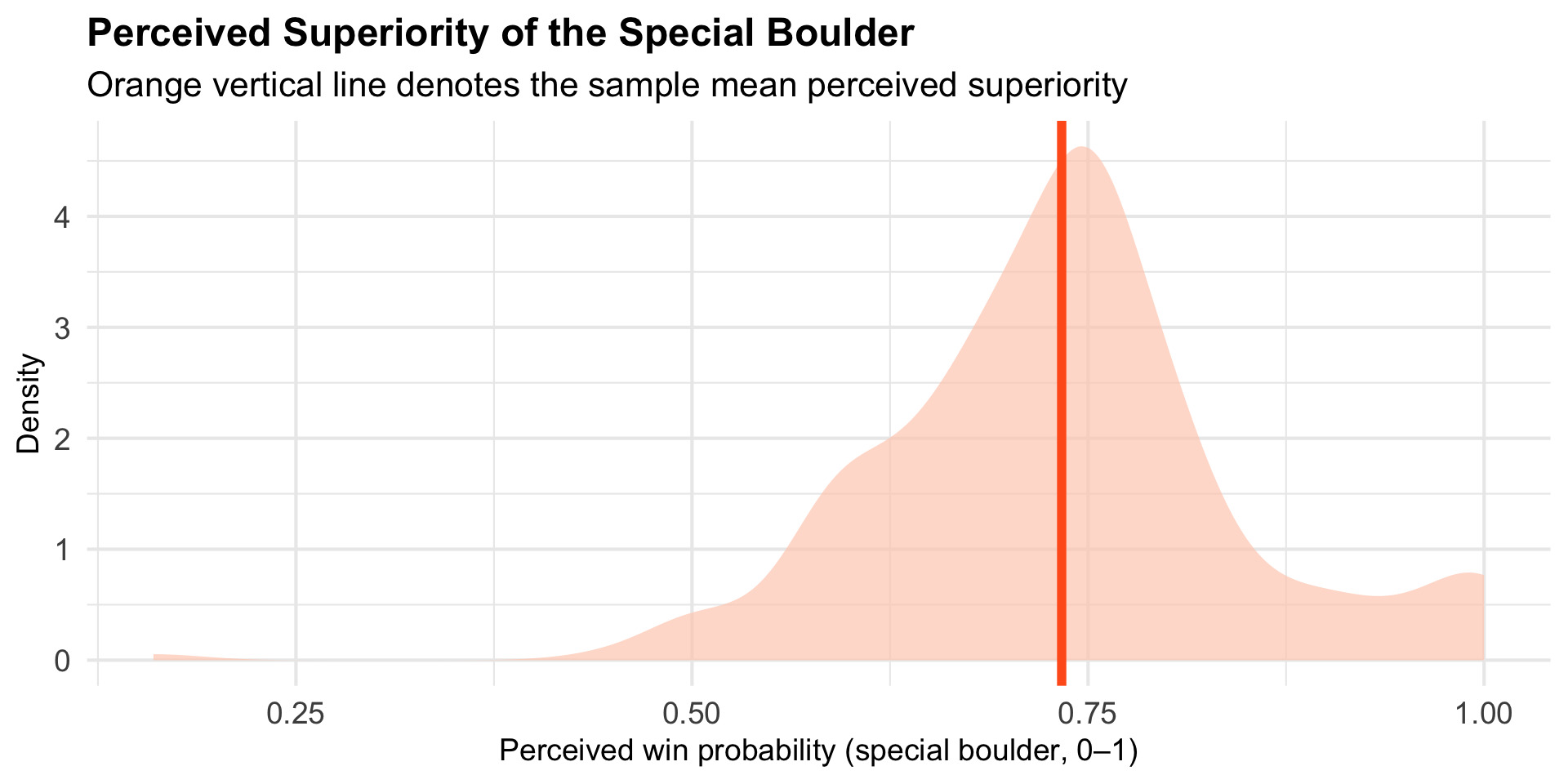
Let’s focus on the PI condition.
Research Question
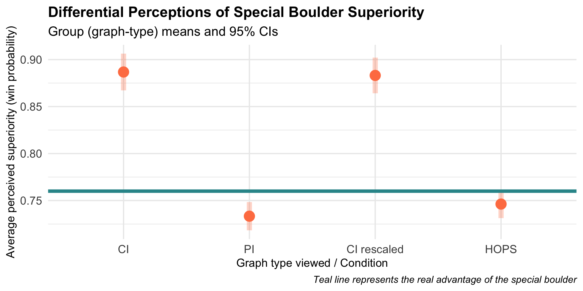
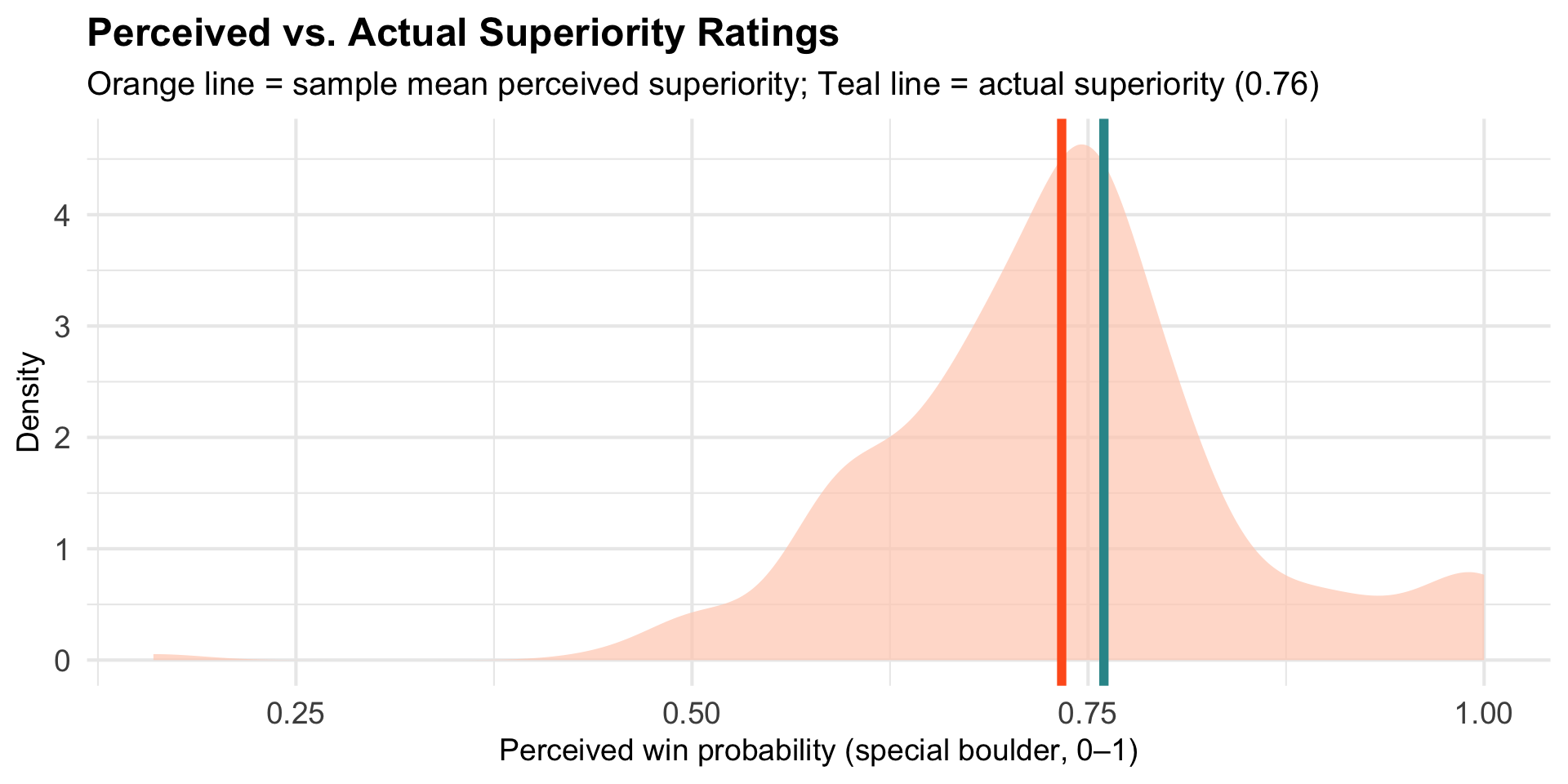
Did participants who saw the PI visualization accurately perceive the boulder’s true advantage (actual winning probability = 0.76) — or did their perceived advantage systematically differ?
Visualize the Raw Data
Overlay the Actual Superiority
Estimation of the Population Parameter
Using our sample, we can estimate the population parameter of interest.
That is, the true mean perceived win probability in the population, denoted \(\mu\).
How Much Uncertainty Is in This Estimate?
Our sample is ONE realization of the data — each potential sample that we would draw would produce a different mean.
Therefore, we need a method to estimate uncertainty around this mean.
We’ve learned a variety of ways to quantify this uncertainty — for example, we can use bootstrap resampling.
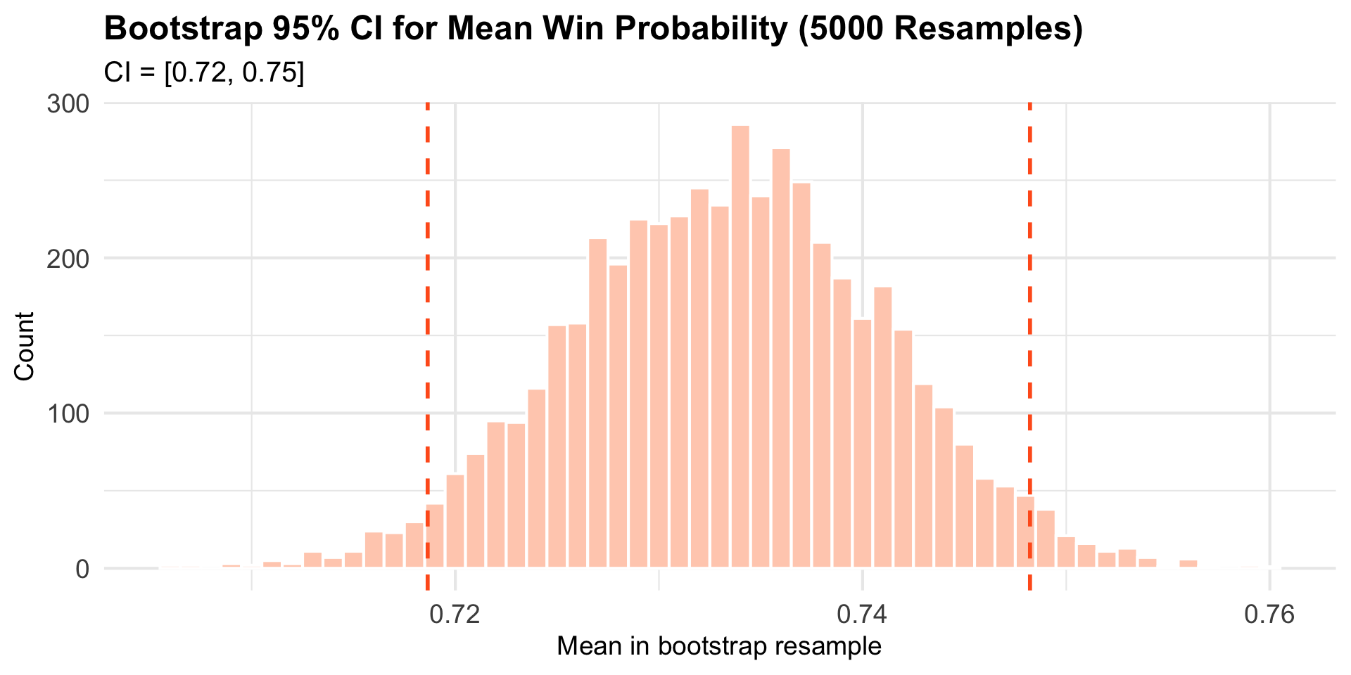
Bootstrap Resampling to Quantify Sampling Variability
Interpretation: We’re 95% confident that the population mean perception of superiority, \(\mu\), lies within this range.
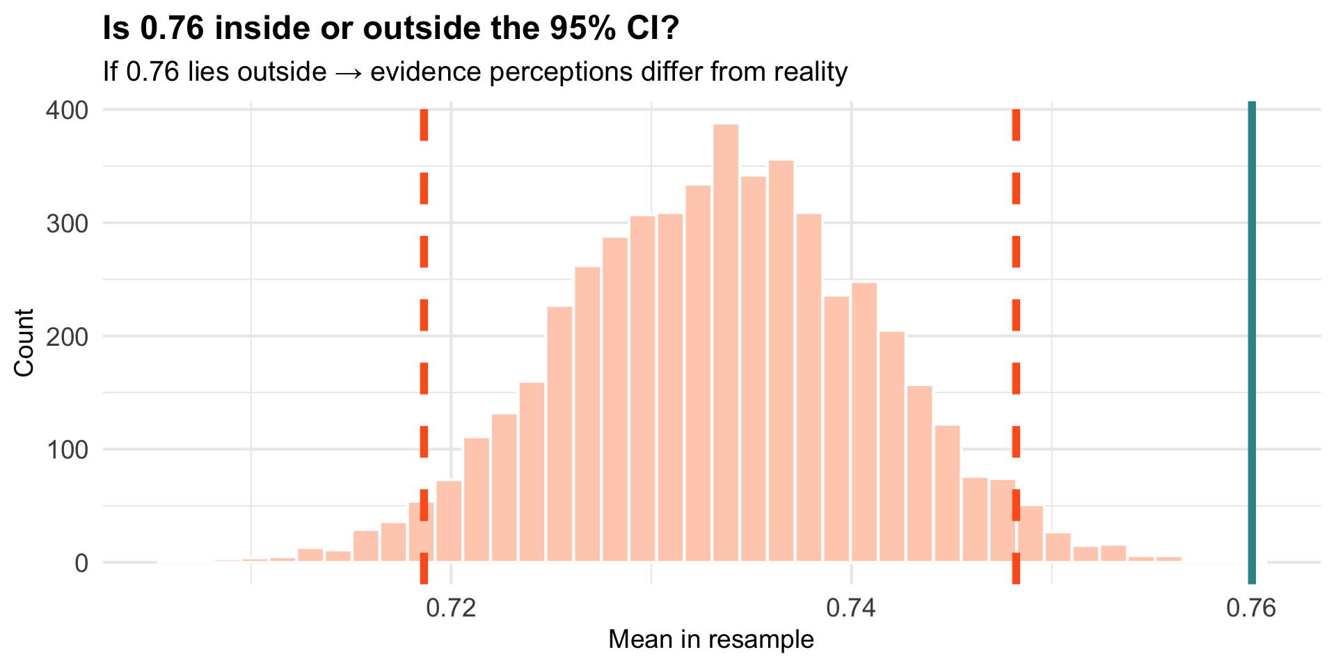
Where Does the Actual Superiority (0.76) Fall?
A Different Question: Starting with a Skeptical Stance
So far: We’ve estimated \(\mu\) and created a CI around our estimate.
Now: What if we start from a position of skepticism?
The Skeptic’s Question
“I think participants perceive the boulder accurately (i.e., \(\mu = 0.76\)). Your sample just happened to be different by chance. Can you prove me wrong?”
This flips our approach: instead of estimating the unknown, we assume a specific value and ask whether our data are compatible with it.
Null Hypothesis Significance Testing (NHST)
The Logic:
State a “null hypothesis” (\(H_0\)): a specific claim about the population we’ll test
State an “alternative hypothesis” (\(H_A\)): what we suspect instead
Assume\(H_0\) is true, then ask: “How surprising is our sample under this assumption?”
If our sample would be very rare under \(H_0\), we have evidence against it
\(H_A\): \(\mu \neq 0.76\): Participants’ perceptions systematically differ from reality.
Key insight: We’re not estimating \(\mu\) anymore — we’re testing a specific claim about what \(\mu\) equals. We’ll refer to this null hypothesis value as \(\mu_0\).
The Core Question of NHST
The Question
IF the null hypothesis were true (i.e., people really do perceive accurately, so \(\mu = 0.76\))…
HOW LIKELY would it be to observe a sample mean as far from 0.76 as ours (\(\bar{x}\) = 0.73)?
To answer this, we need to know what sample means would look like if \(H_0\) were true.
Visualizing the Null World
We already created a bootstrap sampling distribution that shows the variability we’d expect in sample means, centered at our observed mean.
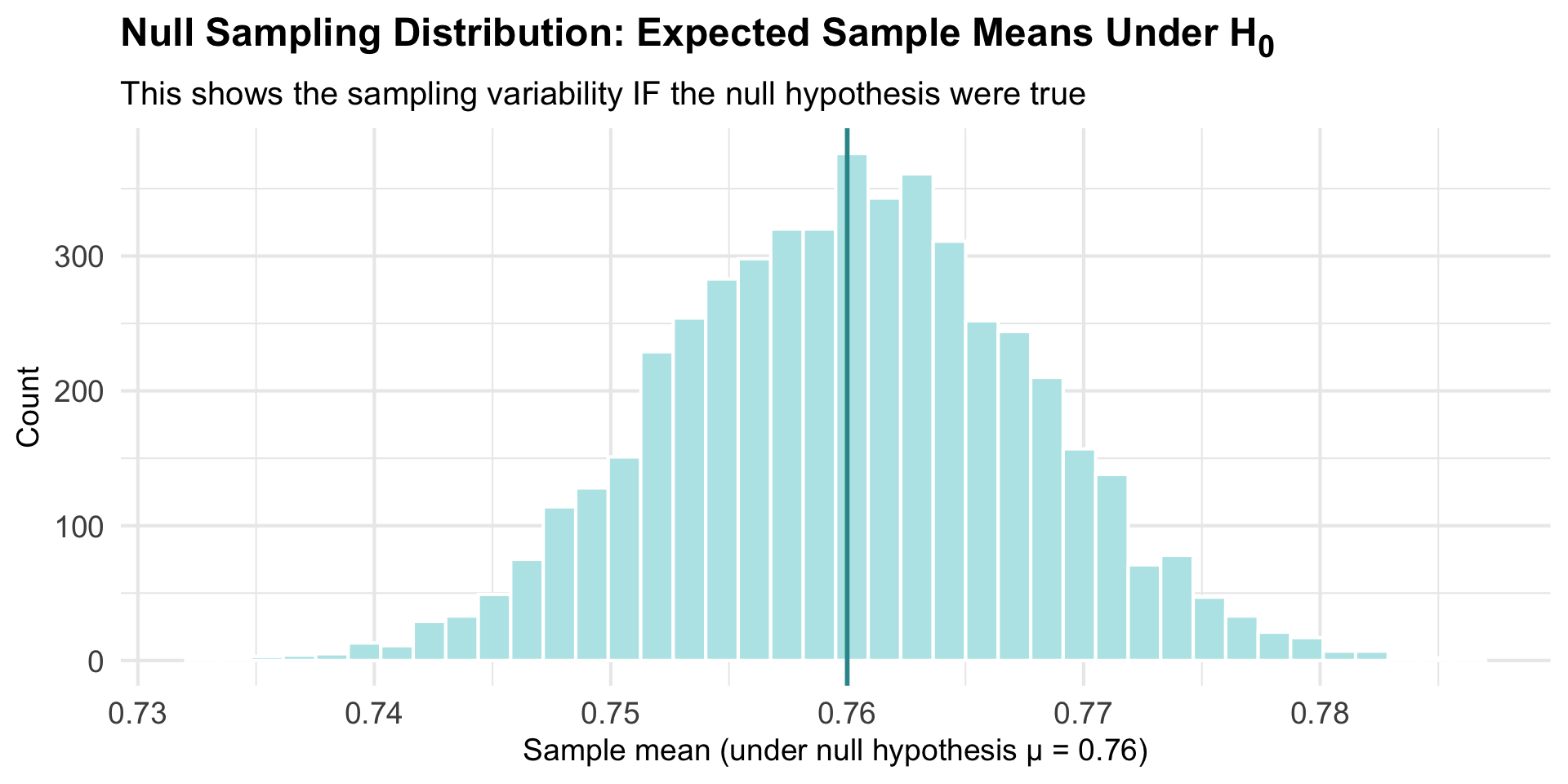
Here’s the key question: What would this sampling distribution look like if the null hypothesis were true — that is, if the true population mean were actually 0.76?
Simple answer: We just shift our entire bootstrap distribution to be centered at 0.76!
The Sampling Distribution Under the Null Hypothesis
This is our “null sampling distribution” — what sample means look like when \(H_0\) is true.
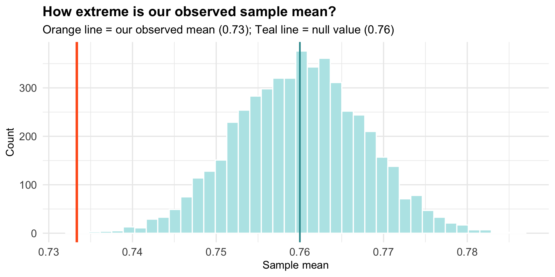
Where Does Our Actual Sample Fall?
Our observed mean (\(\bar{x}\) = 0.73) seems unusual under the null hypothesis.
Quantifying “How Unusual”: The p-value
Important
The p-value is the probability of observing a sample statistic as extreme or more extreme than what we actually observed, assuming \(H_0\) is true.
It is a conditional probability:\[P(\text{data as extreme or more} \mid H_0 \text{ is true})\]
This reads as: “The probability of getting data this extreme (or more), given that the null hypothesis is true.”
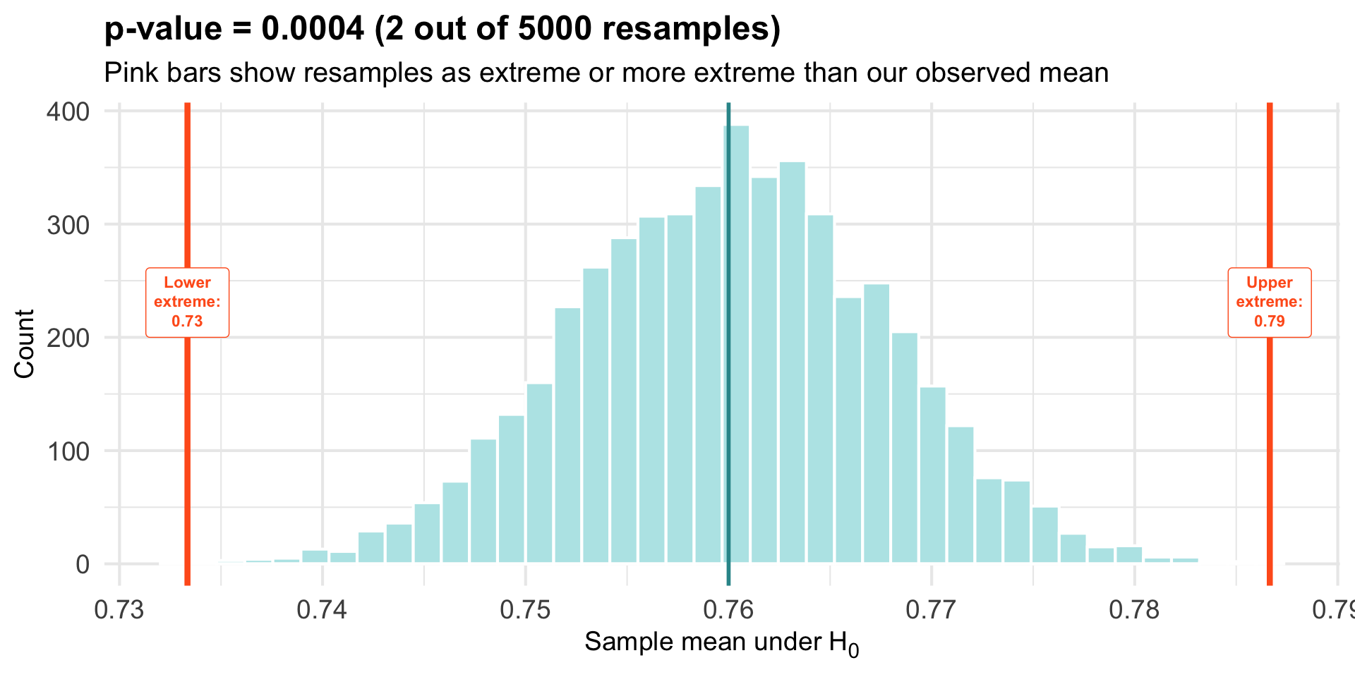
We can count the number of bootstrap resamples from the null world that produce an estimate as extreme or more extreme than our observed sample, and compute the proportion. This is the p-value.
Graphical Depiction of p-value
Both Tails
We look at both tails of the null distribution because our alternative hypothesis is two-sided — we’re testing whether the observed sample mean is either much smaller or much larger than what we would expect if the null hypothesis were true.
The bounds for these regions were computed by taking the null mean (μ₀) and moving an equal distance to the left and right, based on how far the observed mean is from μ₀:
Lower bound = μ₀ − |observed mean − μ₀|
Upper bound = μ₀ + |observed mean − μ₀|
This ensures both tails capture outcomes that are at least as extreme as what we actually observed, regardless of whether the deviation was above or below the null mean.
Interpreting the p-value
p = 0.0004
Interpretation
If the null hypothesis were true (participants perceive accurately), we’d observe a sample mean as extreme as ours in only about 0.04% of samples.
This is quite rare — suggesting our data are not very compatible with the null hypothesis.
Conventional threshold: If \(p < 0.05\), we typically conclude there’s sufficient evidence to reject\(H_0\).
The Connection to Our CI Approach
Notice the parallel logic:
Estimation Approach
NHST Approach
Create CI around our estimate
Create null sampling distribution around hypothesized value
Check if 0.76 falls outside the CI
Check if our sample falls in the extreme tail of null sampling distribution
0.76 is outside the CI → evidence of difference
p < 0.05 → evidence against the null
Both approaches reach the same conclusion — just asking the question differently!
What Could Go Wrong? Four Possibilities
When we make a decision based on our data, there are four possible outcomes:
Reality:\(H_0\) is TRUE
Reality:\(H_0\) is FALSE
Decision: Reject\(H_0\)
❌ Type I Error (False Positive)
✅ Correct Decision (True Positive)
Decision: Fail to Reject\(H_0\)
✅ Correct Decision (True Negative)
❌ Type II Error (False Negative)
We can never know for certain which scenario we’re in — but we can control how often we make errors.
Type I Error: Crying Wolf
Type I Error (α)
Rejecting\(H_0\) when it’s actually true
In our study: Concluding perceptions differ from reality when they actually don’t.
Example: The null is true (\(\mu = 0.76\)), but we happened to get an unusual sample just by chance, leading us to incorrectly reject \(H_0\).
We control the Type I error rate by setting a threshold called alpha(α).
Connection to confidence intervals: When we set α = 0.05 for hypothesis testing, this corresponds to using a 95% confidence interval for estimation. Both approaches use the same threshold — keeping the most extreme 5% (2.5% in each tail) as our criterion for “unusual” results.
Setting Alpha
Alpha (α): The Significance Level
α = maximum Type I error rate we’re willing to tolerate
Convention: α = 0.05 (two-tailed). Should be selected based on the study scenario and should always be set a priori.
What this means: If the null hypothesis is true, we’re willing to incorrectly reject it in at most 5% of studies.
This is why we compare p-values to 0.05:
When α = 0.05:
If \(p < 0.05\): Reject \(H_0\) (result is “statistically significant”)
If \(p \geq 0.05\): Fail to reject \(H_0\)
Type II Error: Missing a Real Effect
Type II Error (β)
Failing to reject\(H_0\) when it’s actually false
In our study: Concluding perceptions are accurate when they actually differ.
Power = 1 - β = probability of correctly detecting an effect when it exists
Type II errors are harder to control directly, but we can reduce them by:
Increasing sample size
Using more precise measurements
Having a larger true effect size
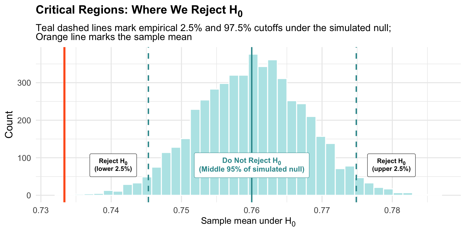
Visualizing Alpha on Our Null Sampling Distribution
Our observed mean (orange) falls in the rejection region → statistically significant.
The Problem: Different Studies Need Different Null Sampling Distributions
Each research question has its own:
Null hypothesis value (0.76, 0, 100, etc.)
Sample size
Variability
Challenge: Hard to compare results across studies or build general rules.
Solution: Use a standardized scale that works for any research question!
Standardization: Creating a Universal Scale
Key insight: Instead of looking at raw means, express how far our sample is from \(H_0\)in standard error units.
To do this, we calculate the standard deviation of the sampling distribution (i.e., the standard error):
Mean in sample: 0.7333
Standard Error (SE): (The standard deviation of the sampling distribution) 0.0077
Our sample mean is about 3.48 standard errors away from the null value. We commonly refer to this standardized difference as the t-statistic or t-ratio.
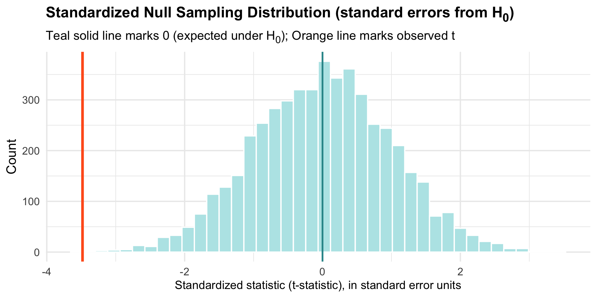
Standardizing the Null Sampling Distribution
Advantage: Now centered at 0 with a standard scale we can use universally!
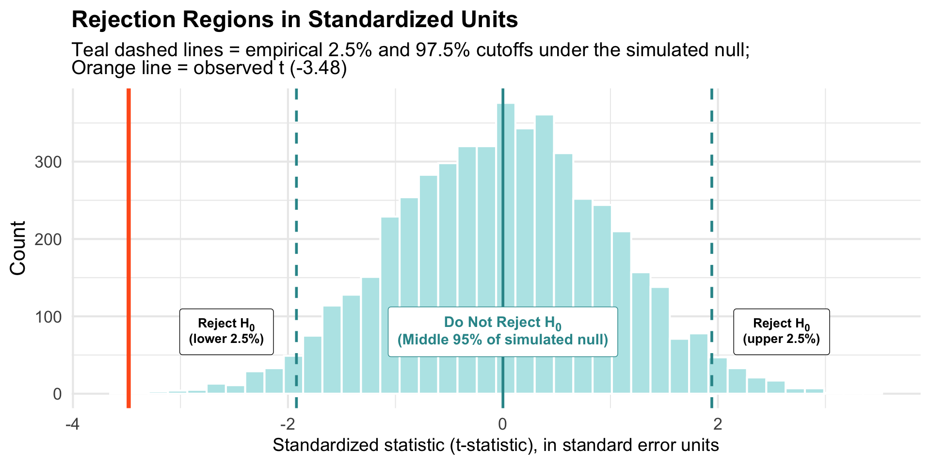
Critical Regions on the Standardized Scale
The Mathematical Shortcut: Student’s t-Distribution
Good news: Under certain assumptions, we don’t need simulation!
Key Assumptions
Random sampling from the population
Independence between observations
Normality: Population is normally distributed (or large sample via Central Limit Theorem (CLT))
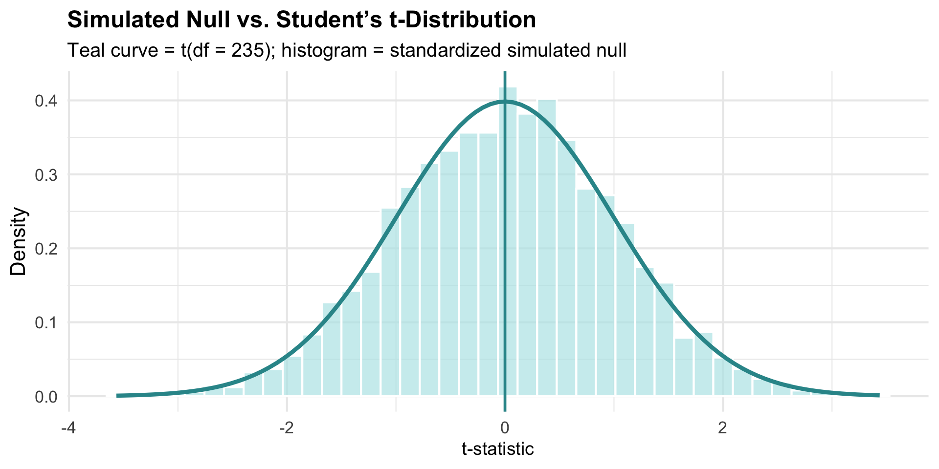
When these hold, the standardized null sampling distribution follows a known mathematical form: Student’s t-distribution with \(df = n - 1\) degrees of freedom (for estimating a population mean).
Comparing Simulated vs. Theoretical Distribution
They match closely.
The Parametric Approach: No Simulation Needed
Instead of bootstrapping to find SE, we can calculate it directly. For a mean:
\[SE(\bar{x}) = \frac{s}{\sqrt{n}}\]
where \(s\) is the sample standard deviation, and \(n\) is the sample size.
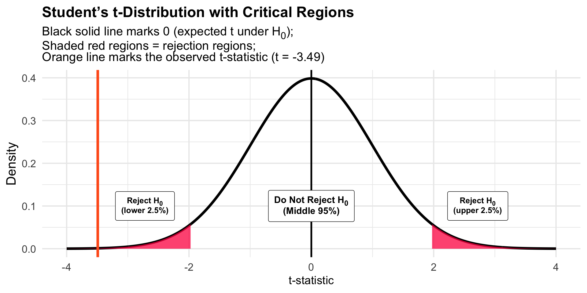
Interpretation: The probability of observing a t-statistic as extreme as -3.49 (or more extreme in either direction) is 0.000574 if the null hypothesis were true.
A One-Sample t-test
Interpretation:
\(t(235) = -3.49\), \(p = 0.00057\)
Our observed mean (0.733) is significantly different from 0.76
95% CI: [0.72, 0.75]
Conclusion: Participants who saw the PI visualization underestimated the special boulder’s advantage.
Summary: The NHST Framework
The complete process:
State hypotheses:\(H_0\) vs. \(H_A\)
Set α level (often 0.05 — two-tailed — with 0.025 in each tail)
Calculate test statistic
Find critical values using qt() and/or calculate p-value using pt()
Make decision:
If \(p < \alpha\) (or \(|t|\) exceeds the critical value): Reject\(H_0\)
If \(p \geq \alpha\) (or \(|t|\) does not exceed the critical value): Fail to reject\(H_0\)
Key insight: A 95% CI that excludes the null value, a p-value < 0.05, and a t-statistic in the rejection region all tell the same story!
Wrapping Up
Remember:
NHST starts with a skeptical stance (the null hypothesis)
We evaluate whether our data would be surprising under that assumption
Standardization allows us to compare results across different studies
The t-distribution provides a theoretical shortcut when assumptions hold
The p-value is NOT the probability that the null hypothesis is true — it is the probability of obtaining a test statistic as extreme or more extreme than in the observed sample, IF the null hypothesis is true.