PSY 652: Research Methods in Psychology I
Fitting Non-Linear Relationships with lm()
Kimberly L. Henry: kim.henry@colostate.edu
The data
In lab you’ve been exploring data from a paper which examines hidden biases in criminal sentencing.

Specifying the Functional Form of the Control Variables
Blair and colleagues hypothesized that sentence length should exhibit a non-linear, ramping up pattern as the seriousness of the offense increases:
- At low levels of seriousness → each one-unit increase should have a small increasing effect on sentence length (theft < $5K → theft $5K-$10K)
- At high levels of seriousness → each one-unit increase should have a larger increasing effect on sentence length (assult → murder)
Translation: The effect of offense severity should accelerate as severity increases (i.e. a non-linear relationship).
Import the Data
Key Variables:
- years: Sentence length in years (outcome)
- primlev: Severity of primary offense (predictor, scale 1-11)
Explore the Outcome: Sentence Length in Years
Tip
Problem: The distribution is highly right-skewed (i.e., positive skew).
Initial Look: Severity → Years
Tip
The relationship appears positive, but the linear best-fit line does not capture the pattern well.
Why Is Skewness a Problem?
- Likely creates non-normality of residuals (normally distributed residuals is an assumption of a fitted model)
- Outliers have disproportionate influence on the model
- Heteroscedasticity: Variance of residuals often increases with fitted values (the residual standard deviation — sigma — is assumed to be adequate at all levels of the fitted values.
- Poor fit to the data: Linear effects may not capture the multiplicative nature of the relationship
Solution: Transform the outcome using the natural logarithm!
The Log Transformation
Create a new variable lnyears that is the natural log of years:
Tip
Still skewed, but much better!
After Log Transform: Severity → ln(years)
Tip
This is much better! But, Blair and colleagues hypothesized a quadratic curve.
Can a Quadratic Model do Better?
Tip
The quadratic curve seems like it is a better fit.
Testing for Non-Linearity: Two Models
Let’s compare the linear fitted model to a quadratic fitted model:
Adding the Quadratic Term
Tip
Key observations:
The quadratic term (
I(primlev^2)) is reliably different from zeroR² increases from the linear model (about 0.45 to 0.50)
Interpreting the Quadratic Model Coefficients
Model: \({lnyears} = {b_0} + ({b_1} \times {primlev_i}) + ({b_2}\times {primlev_i^2})\)
- \({b_0}\) (intercept): Expected/predicted ln(years) when offense severity = 0
- \({b_1}\) (primlev): The initial rate of change (slope at primlev = 0)
- \({b_2}\) (primlev²): How the slope changes as primlev increases
- If \({b_2}\) > 0 (positive): Accelerating relationship (bowl-shaped)
- If \({b_2}\) < 0 (negative): Decelerating relationship (mound-shaped)
Important:
The predictor, primlev, doesn’t have a meaningful 0 (1 is the lowest score). We’ll ignore this here to keep things simple — but when you replicate the five models from the Blair paper later, we’ll center this and all other predictors.
Individual coefficients in polynomial models are best interpreted using marginal effects!
The equation for the fitted model
\[ \hat{lnyears} = {b_0} + ({b_1} \times {primlev_i}) + ({b_2}\times {primlev_i^2}) \] \[ \hat{lnyears} = 0.765 + (-0.289 \times {primlev_i}) + (0.048\times {primlev_i^2}) \] What is the predicted score when severity equals 6?
\[ \hat{lnyears} = 0.765 + (-0.289 \times 6) + (0.048\times {6^2}) \approx 0.75 \]
Computing Predictions with marginaleffects
Let’s request predictions of ln(years) with 95% CIs at each level of severity:
Tip
These predictions are on the log scale — ln(years).
Visualizing Predictions: ln(years) Scale
Tip
Notice the accelerating curve and widening confidence intervals at the extremes.
Back-Transforming to Original Scale: Sentence Length in Years
To interpret predictions in years — not ln(years) — we exponentiate:
Tip
Key point: We exponentiate the predictions AND both confidence bounds.
Visualizing Predictions: Years Scale
Tip
Now we see predictions in meaningful units! The exponential transformation makes the curve even steeper.
Understanding Marginal Slopes
Problem: In polynomial models, the effect of X on Y varies depending on the value of X.
Question: “What is the effect of a one-unit increase in offense severity?”
Answer: “It depends on the current level of severity!”
- At severity = 4, increasing by 1 might add a couple months to the sentence
- At severity = 10, increasing by 1 might add well over 10 years
Solution: Calculate marginal effects (slopes) at specific values of the predictor.
Computing Marginal Effects (Slopes)
We’ll calculate slopes at three levels of offense severity: 3, 6, and 9
\[ {b_1} + (2\times{b_2}\times{primlev_i}) \]
\[ {-0.28919004} + (2\times{0.04784813}\times{primlev_i}) \] Hand computation when severity equals 6:
\[ {-0.28919004} + (2\times{0.04784813}\times{6}) \approx 0.285 \]
Tip
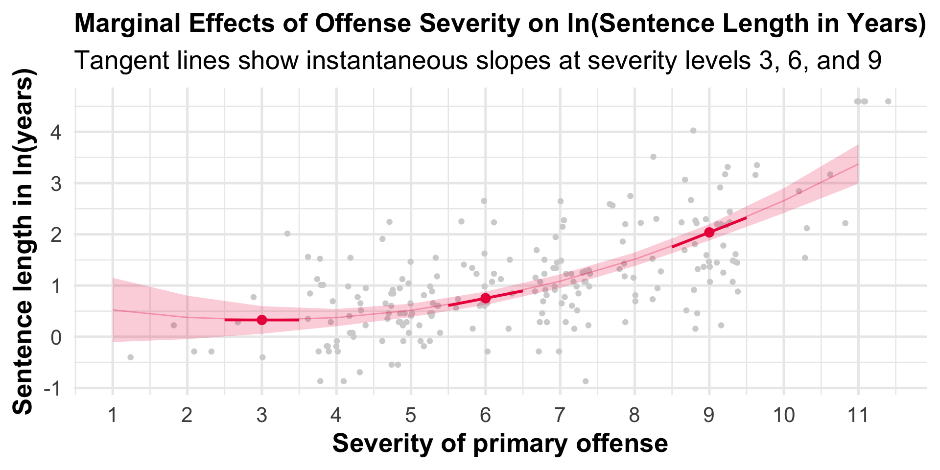
Interpretation: These are slopes on the ln(years) scale. Notice how the slope increases as primlev increases!
What Do These Slopes Mean?
The estimate column shows the instantaneous slope at each value of primlev.
At primlev = 3: slope ≈ -0.002: A 1-unit increase in severity doesn’t substantially change ln(years)
At primlev = 6: slope ≈ 0.285: A 1-unit increase in severity increases ln(years) by 0.285 units
At primlev = 9: slope ≈ 0.572: A 1-unit increase in severity increases ln(years) by 0.572 units
Pattern: The effect of offense severity accelerates as severity increases (supporting the hypothesis!).
Visualizing Slopes: ln(years) Scale
Converting Slopes to Percent Changes
If we want to interpret effects on the original metric (years), we can convert the coefficients to percent changes using the formula: 100 × (exp(β) - 1). This gives us the percent change in sentence length (in years) for a one-unit increase in severity. This formula is enacted in the function below.
Tip
When the primary offense is level 6 severity, a 1-unit increase in severity equate to ~33.0% increase in sentence length in years.
Automate the process
Tip
Now we have percent changes at each severity level!
Interpreting Percent Changes
At primlev = 3: A 1-unit increase in severity → ~ (-.2%) decrease in sentence length in years (though CI includes 0)
At primlev = 6: A 1-unit increase in severity → ~33.0% increase in sentence length in years
At primlev = 9: A 1-unit increase in severity → ~77.2% increase in sentence length in years
Key finding: The marginal effect of offense severity becomes much larger as we move to more severe offenses! This supports Blair et al.’s hypothesis of an accelerating relationship.
Understanding Slope Magnitude
Percent change tells us the relative effect: “Y increases by 20%”
Slope magnitude tells us the absolute effect: “Y increases by 2 years”
Formula:
Example: At severity = 6, if:
Predicted sentence = 2.1 years
Percent change = 33%
Then slope magnitude = 2.1 × 0.33 = ~ 0.7 years
We need slope magnitude to draw tangent lines on the years scale!
Compute the slope magnitudes
Tip
When primary offense severity = 6, a one unit increase in severity (e.g., going from a 6 to a 7) is expected to increase sentence length by about 0.7 years.
Visualizing Slope Magnitudes: Years Scale
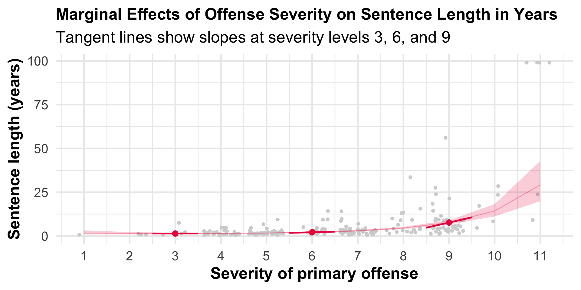
The steepening tangent lines show the accelerating effect in absolute terms (years).
Summary: Key Takeaways
- Log transformations normalize skewed outcomes and enable percent interpretations
- Polynomial regression captures non-linear relationships (like accelerating effects)
- Marginal effects helps in interpreting complex models
- Visualization helps communicate findings