PSY 652: Research Methods in Psychology I
Continuous Probability Distributions
Kimberly L. Henry: kim.henry@colostate.edu
The data
We’ll consider data that covers the modern Olympic Games, from Athens 1896 to Rio 2016. The data were originally scraped from www.sports-reference.com. It was then formatted for data analysis by Kaggle, a popular platform for data science competitions.
Variables
| id |
double |
Athlete ID |
| name |
character |
Athlete name |
| sex |
character |
Athlete sex |
| age |
double |
Athlete age |
| height |
double |
Athlete height in cm |
| weight |
double |
Athlete weight in kg |
| team |
character |
Country/Team competing for |
| noc |
character |
NOC region |
| games |
character |
Olympic Games name |
| year |
double |
Year of Olympics |
| season |
character |
Season (either Winter or Summer) |
| city |
character |
City of Olympic host |
| sport |
character |
Sport |
| event |
character |
Specific event |
| medal |
character |
Medal (Gold, Silver, Bronze) |
Import the data
Let’s import the data:
A small subset of the data
Here’s a subset of the data for you to peruse.
What is a Probability Density Function?
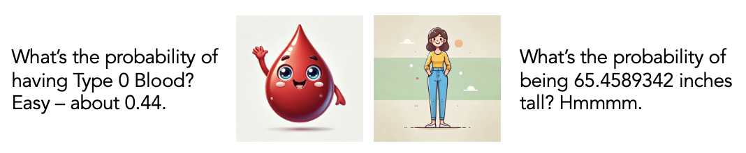
A probability density function (PDF) is used to describe the distribution of a continuous random variable.
Unlike a discrete variable, where we can directly calculate the probability of specific outcomes using a PMF (e.g., the probability that a news article is fake), a PDF represents the probability that a continuous variable falls within a particular interval.
The PDF is a smooth curve describing how “dense” the probability is in different regions.
![An image of a blood drop with the caption: What's the probability of having Type O blood? Easy - about 0.44. And, an image of a woman with the caption: What's the probability of being 65.4589342 inches tall? Hmmm]()
Why do we need a different function?
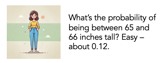
For a continuous variable, the probability of the variable taking any exact value is technically zero, because there are infinitely many possible values it could take.
Instead, the PDF helps us calculate the probability that the variable falls within an interval.
The area under the curve of the PDF over a given range represents the probability of the variable being in that interval.
![An image of a woman with the caption: What's the probability of being between 65 and 66 inches tall? Easy -- about 0.12.]()
An example empirical PDF
The Olympics data provides the height and weight for each athlete, and from this, we can calculate the body mass index (BMI) — which is a continuous random variable.
Let’s compute the BMI for the male athletes.
We will create a subsetted data frame called male_athletes — in this data frame we will keep only the athlete’s first appearance in the Olympic Games (if they were in multiple).
BMI is computed as:
\[
BMI = \frac{weight\ (\text{kg})}{\left(\frac{height\ (\text{cm})}{100}\right)^2}
\]
Create data frame
There are a couple of new functions in this code. First, distinct(id, year, .keep_all = TRUE) removes duplicates for each athlete (id) in the same year (year), ensuring that only one row per athlete per Olympic year is retained, even if the athlete participated in multiple events. The keep_all argument ensures all columns are retained in the result, not just the columns specified in distinct(). Second, slice_min(order_by = year, n = 1) selects the earliest (smallest/minimum) year for each athlete (the first Olympic Games they participated in).
Create an empirical PDF of BMI for males
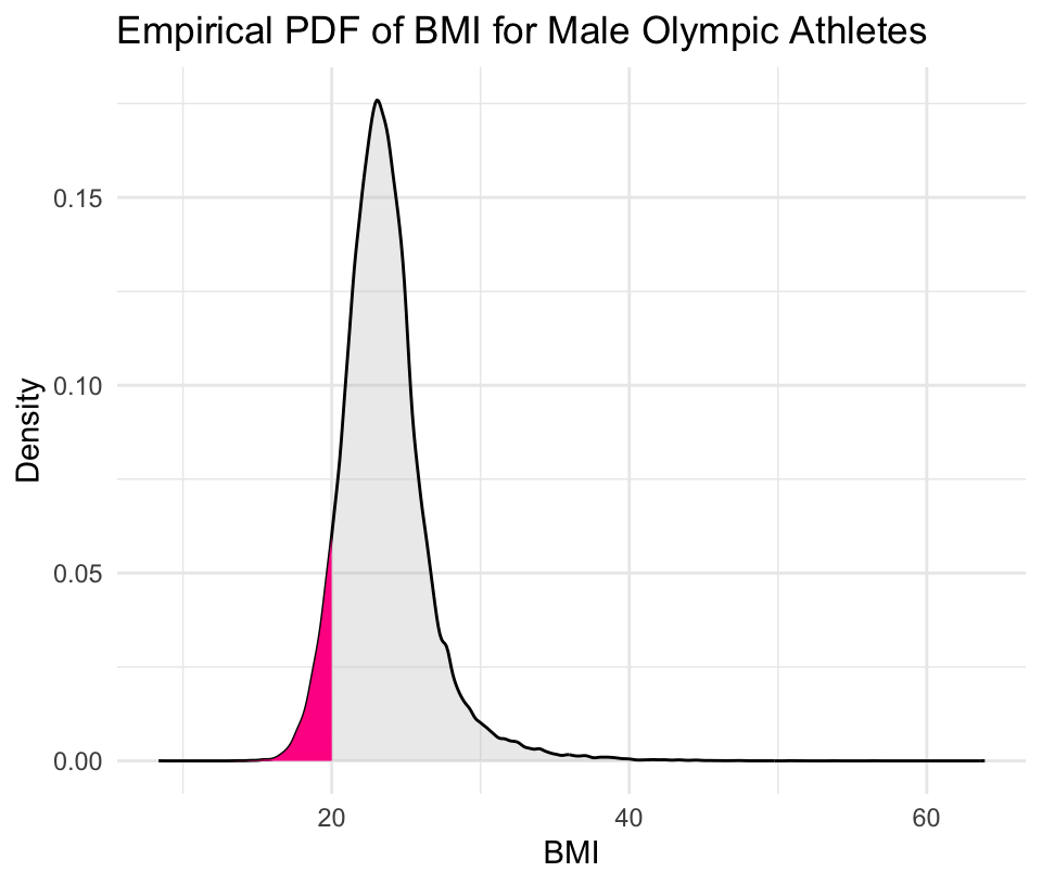
A density plot is the visualization of the empirical PDF.
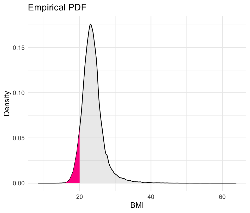
PDF of all male athletes, \(P(\text{BMI} \le 20)\) is highlighted
![An image of the PDF of BMI (BMI <= 20 is marked)]()
The Cumulative Distribution Function (CDF)
The CDF answers the question: “What’s the probability of getting a value this small or smaller?”
- For any point on your distribution, the CDF tells you the probability that a randomly selected value falls at or below that point
- Think of it as a running total of probabilities as you move from left to right along the distribution
- Visually, the CDF value equals the total area under the curve to the left of your chosen point
Calculate and plot the empirical CDF
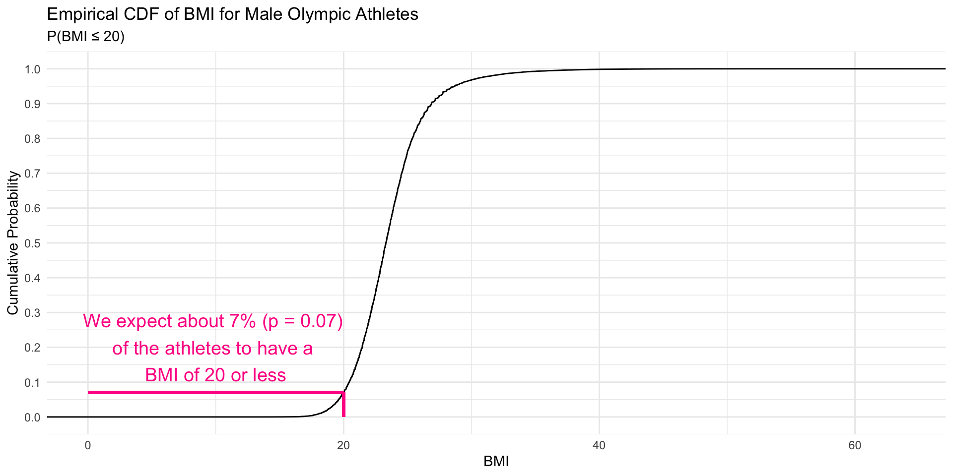
The stat_ecdf() function in ggplot2 computes the empirical CDF for a given variable, in this case, the BMI of male athletes. It shows the cumulative probability of the variable (BMI) being less than or equal to a given value. For each BMI value on the x-axis, the y-axis shows the proportion of observations that have a BMI less than or equal to that value.
Interpreting the CDF
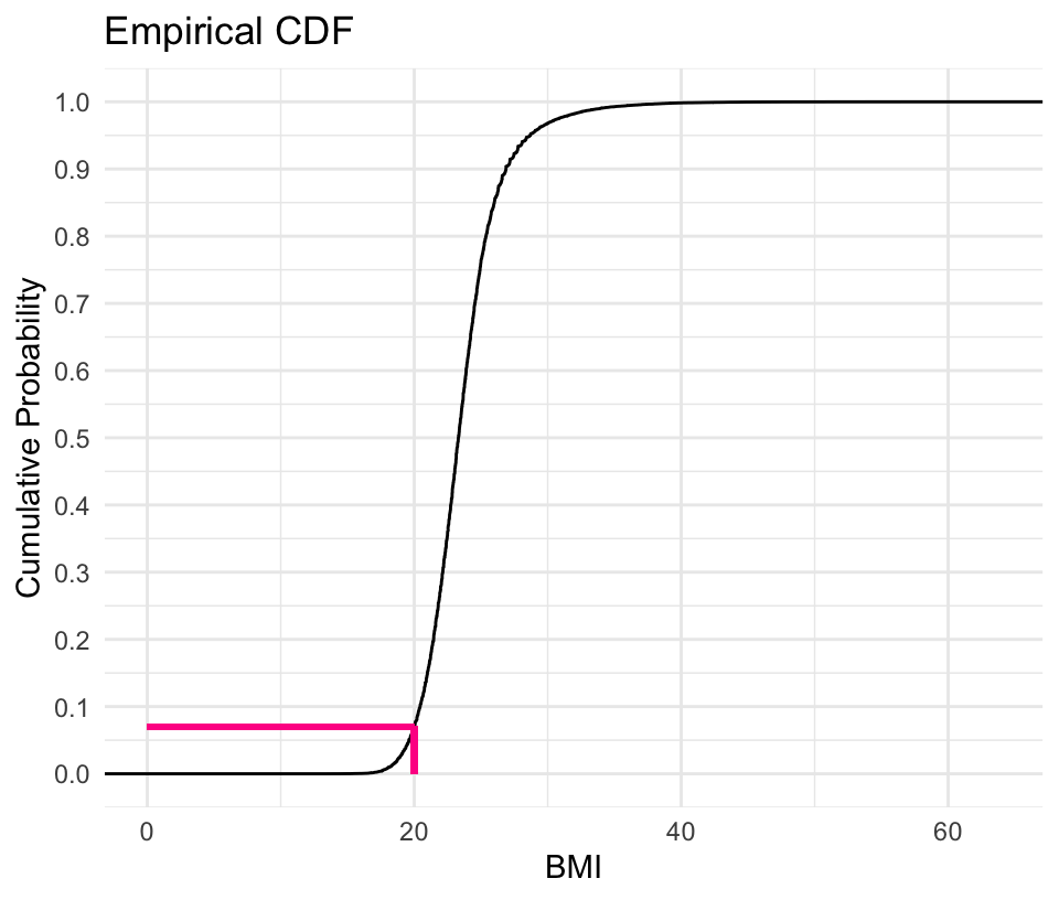
![An image of the CDF of BMI, at x = 20, y = 0.07]()
The value of the CDF function at any point represents the cumulative probability up to that point. The ECDF ranges from 0 to 1, and the y-axis gives the probability that a randomly selected observation is less than or equal to the corresponding x-value.
Comparison of PDF and CDF
The graphs below both display the \(P(\text{BMI} \le 20)\)
PDF (Left Graph): The probability \(P(BMI≤20)\) is represented by the area of the shaded pink region (with respect to the total area under the curve ~ i.e., about 7%).
CDF (Right Graph): The same probability \(P(BMI≤20)\) is represented by the height of the CDF curve at the point where BMI = 20.
Using the distribution to compute probabilities
The ecdf() function in R computes the empirical CDF (ECDF) for a variable — e.g., BMI. This allow us to use the distribution to answer questions about the probability of randomly selecting a case (e.g., a male Olympic athlete) within a certain interval. Press Run Code on the code chunk below to set up the ecdf_bmi() function for this example. Then, we’ll use the function in the next slides.
Compute \(P(\text{BMI} \le 20)\)
By calling the ecdf_bmi() function just created, the code below will return the probability that the BMI of a randomly selected male athlete is less than or equal to 20.
This is the BMI score that we studied on the prior empirical PDF and CDF graphs.
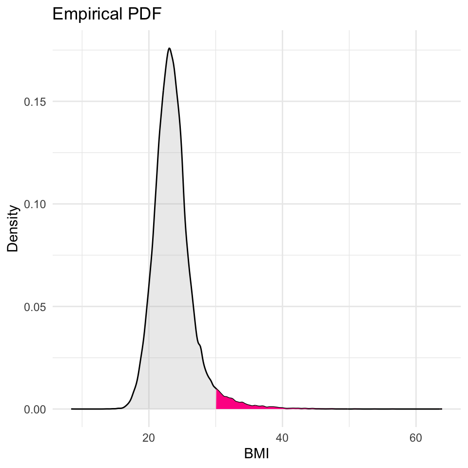
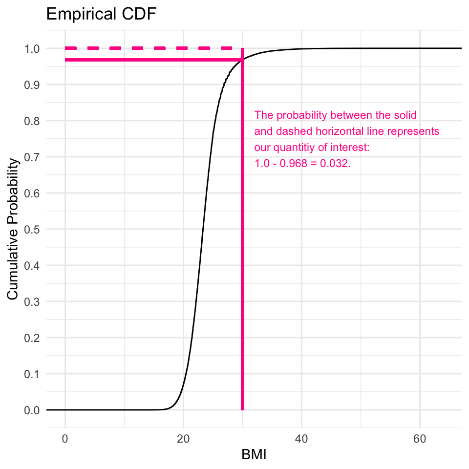
What is the probability of a BMI >= 30?
To solve for this, we leverage the complement of the ECDF for the value 30. The ECDF gives the probability of a BMI being less than or equal to a specified value, so the probability of a BMI being greater than or equal to 30 is:
\[
P(BMI \geq 30) = 1 - P(BMI \leq 30)
\]
Comparison of PDF and CDF
The graphs below both display the \(P(\text{BMI} \ge 30)\)
Practice with ECDF
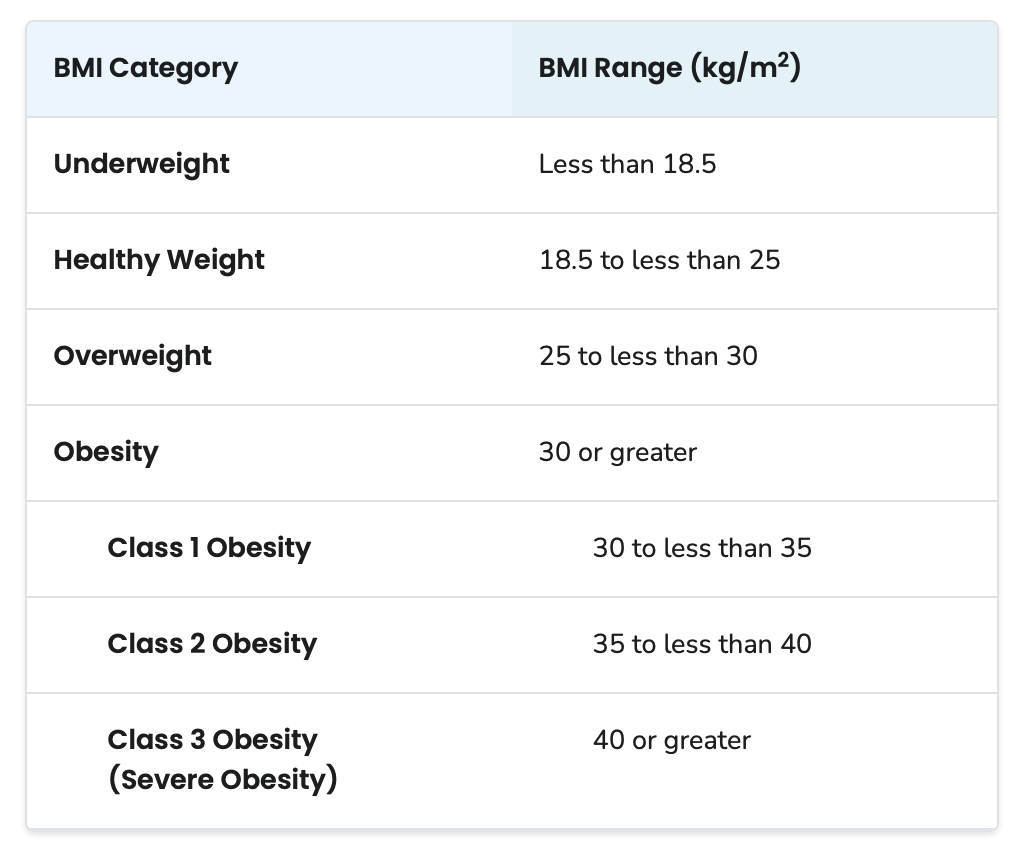
The chart below presents the recommendations for a healthy BMI. Using this chart, please answer the following three questions (next three slides).
![]()
ECDF Q1:
What is the probability that a randomly selected male Olympic athlete will be underweight?
ECDF Q2:
What is the probability that a randomly selected male Olympic athlete will be severely obese?
ECDF Q3:
What is the probability that a randomly selected male Olympic athlete will a healthy weight?
PDF and CDF for the Normal Distribution
Now that we’ve explored the Empirical PDF and Empirical CDF for BMI, which are based on our observed data, let’s move on to understanding the PDF and CDF for a normal distribution.
A normal distribution (also known as a Gaussian distribution) is symmetric, bell-shaped, and is fully described by its mean (center of the distribution) and standard deviation (which controls the spread of the data).
Once we know a variable is normally distributed, we no longer need the raw data to calculate probabilities or understand its distribution.
In short, knowing a variable is normally distributed allows us to leverage the mathematical properties of the distribution to calculate probabilities, rather than needing the original dataset.
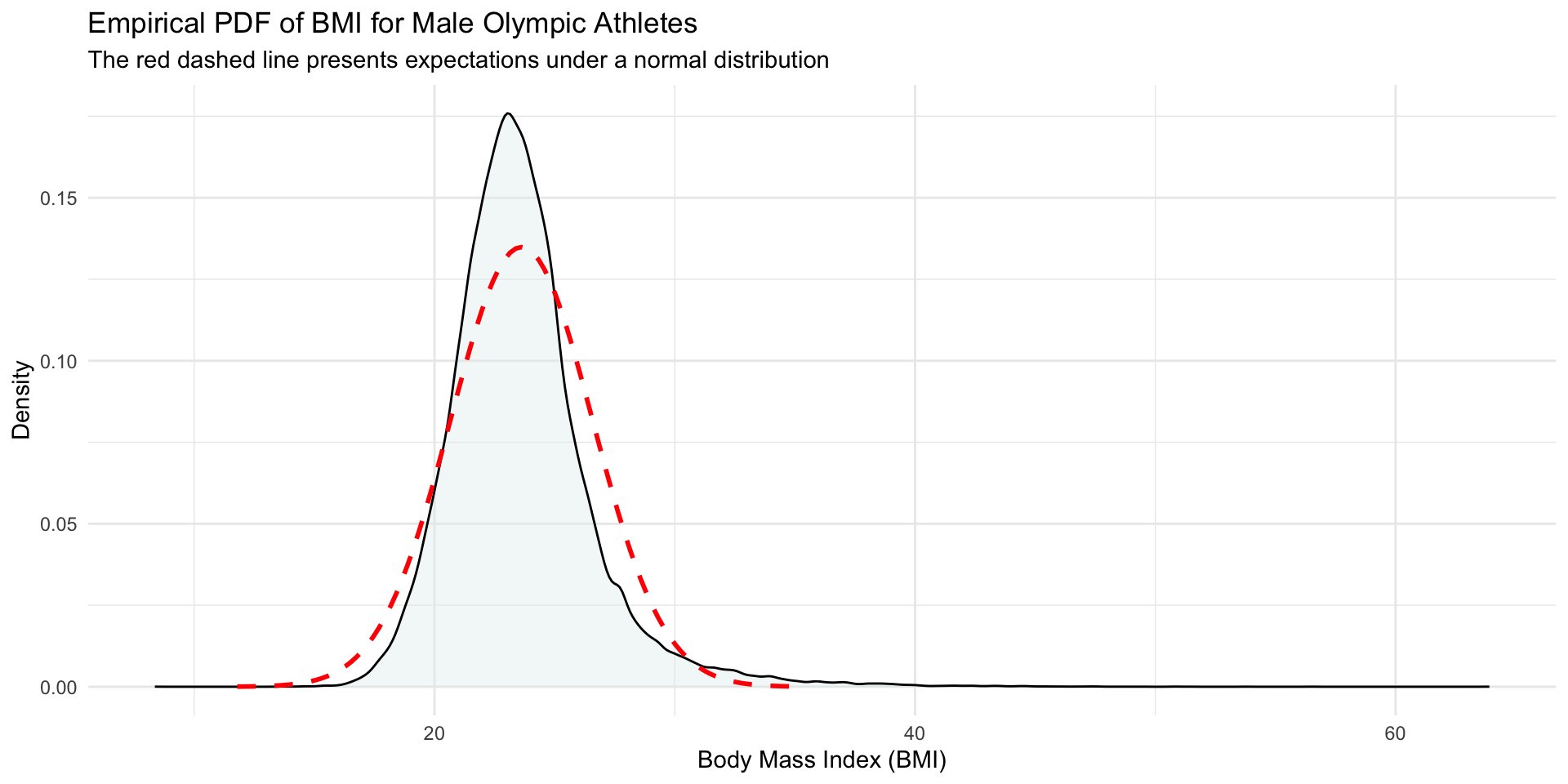
Is BMI of male Olympic athletes normally distributed?
![A dentisy plot of BMI for all male athletes with a normal curve overlaid.]()
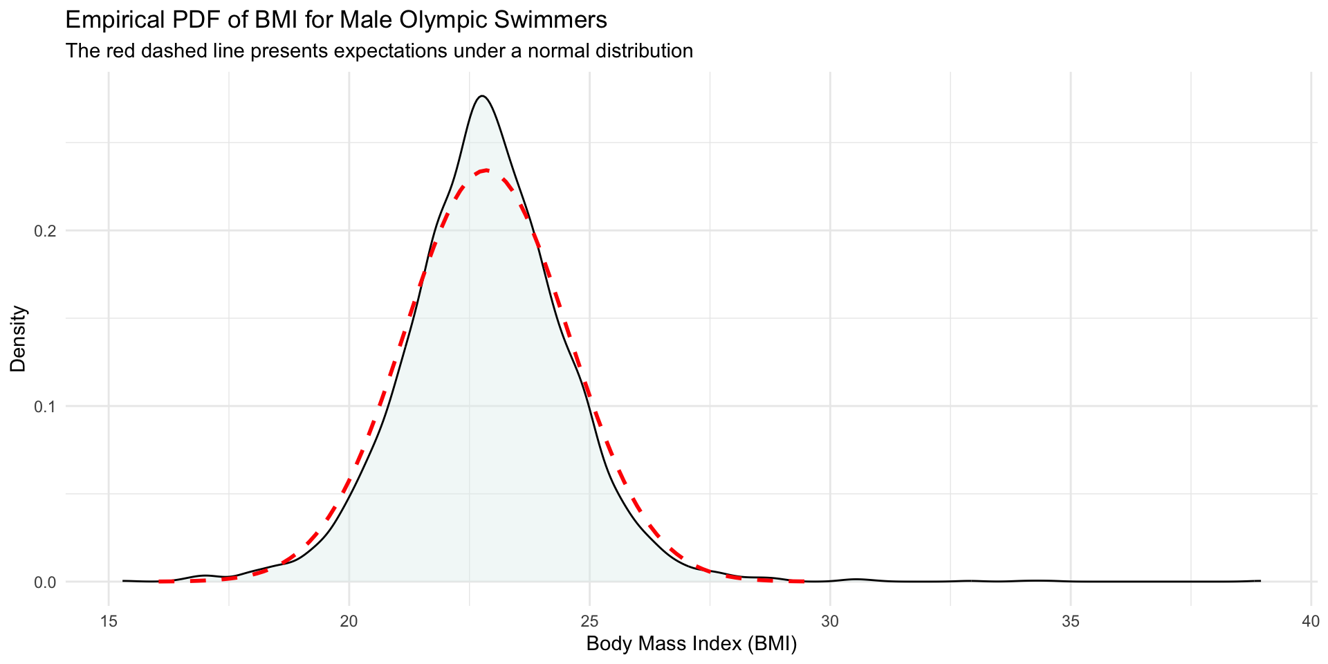
Is BMI of male Olympic swimmers normally distributed?
![A dentisy plot of BMI for male swimmers with a normal curve overlaid.]()
Calculate Mean and Standard Deviation (SD)
Let’s subset the male_athletes data frame to include just swimmers (we’ll call the data frame swimmers), then compute the mean and SD of BMI for this group.
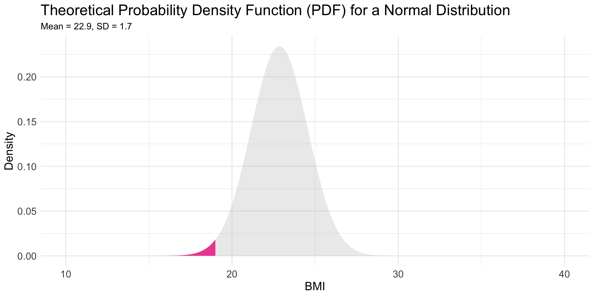
Using the Normal Distribution, what is the probability that a male Olympic swimmer will have a BMI less than or equal to 19?
![Male swimmer BMI with <=19 marked]()
Answer the question using pnorm()
pnorm(q = my_q, mean = my_mean, sd = my_sd)
q: The quantile or value at which to evaluate the CDF (19)
mean: The mean of the normal distribution (22.9)
sd: The standard deviation of the normal distribution (1.7)
- The probability is about 0.01 that a male Olympic swimmer has a BMI of 19 or less. Or, we can say — there is about a 1% chance that a male Olympic swimmer has a BMI of 19 or less.
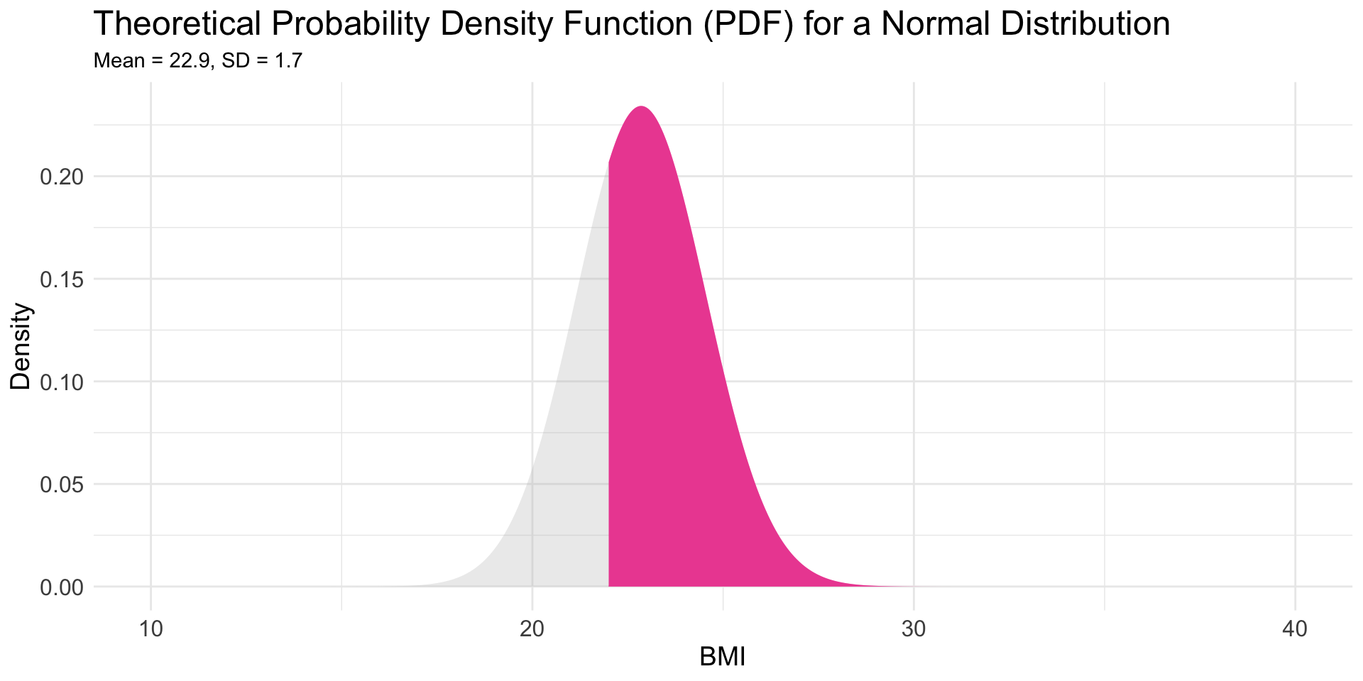
\(P(\text{BMI} \ge 22)\)
What is the probability that a male swimmer will have a BMI greater than or equal to 22?
![Male swimmer BMI with >= 22 marked]()
Answer the question using pnorm()
The lower.tail = FALSE argument in the pnorm() function is necessary when you want to find the upper tail probability (i.e., the probability that a normally distributed variable is greater than a certain value). By default, pnorm() calculates the lower tail probability, meaning it gives you the probability that the random variable X is less than or equal to a specified value q. However, if you are interested in the upper tail, you need to calculate the complement of the lower tail probability. Setting lower.tail = FALSE does this automatically.
- The probability is 0.70 that a male Olympic swimmer has a BMI of 22 or greater.
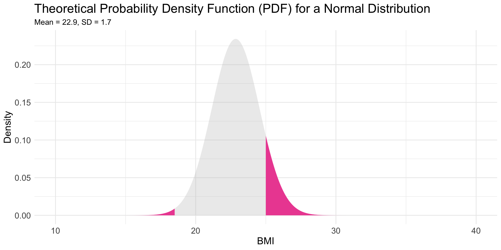
\(P(\text{BMI} \le 18.5)\) or \(P(\text{BMI} \ge 25)\)
What is the probability of a BMI of 18.5 or less OR a BMI of 25 or higher
![Male swimmer BMI with <= 18.5 and >= 25.0 marked]()
Answer the question using pnorm()
Hint — here, we need to sum two probabilities.
- The probability is 0.11 that a male Olympic swimmer has a BMI less than or equal to 18.5 OR greater than or equal to 25.
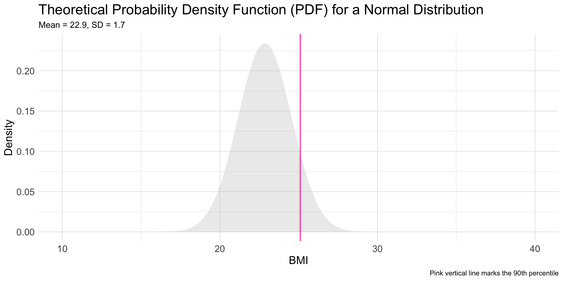
Calculate a quantile from a probability
We might ask a different type of question in this context:
What BMI represents the 90th percentile of the distribution?
For this, we use the qnorm() function — it finds a quantile (q) based on a probability (p).
- A BMI of 25.1 represents the 90th percentile of the distribution. At this point, 90% of the scores fall below and 10% fall above.
A graph to depict the 90th percentile
![A PDF of male swimmers BMI with the 90th percentile marked]()
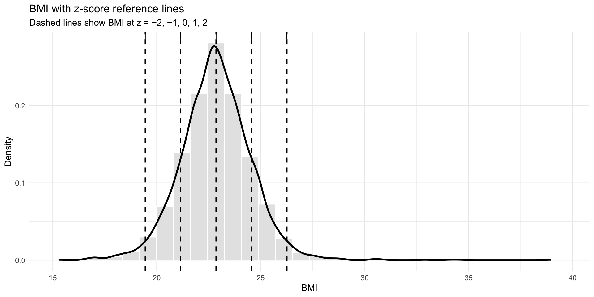
The Standard Normal Distribution
Z-scores for male swimmers
Recall that the standard normal distribution is a normal distribution of z-scores. The code below, creates a z-score for BMI among the male swimmers
The relationship between the raw and z-score
![A histogram that links the raw scores to the z-scores for male swimmers]()
What is the Standard Normal Distribution?
A standard normal distribution is a distribution of z-scores. Recall that a z-score distribution has a mean of 0 and a standard deviation (sd) of 1. A z-score tells you how many standard deviations a value is from the mean.
What scores (i.e., quantiles) of the standard normal distribution mark the middle 95% of the distribution? Here we want to solve quantiles, so we use qnorm().
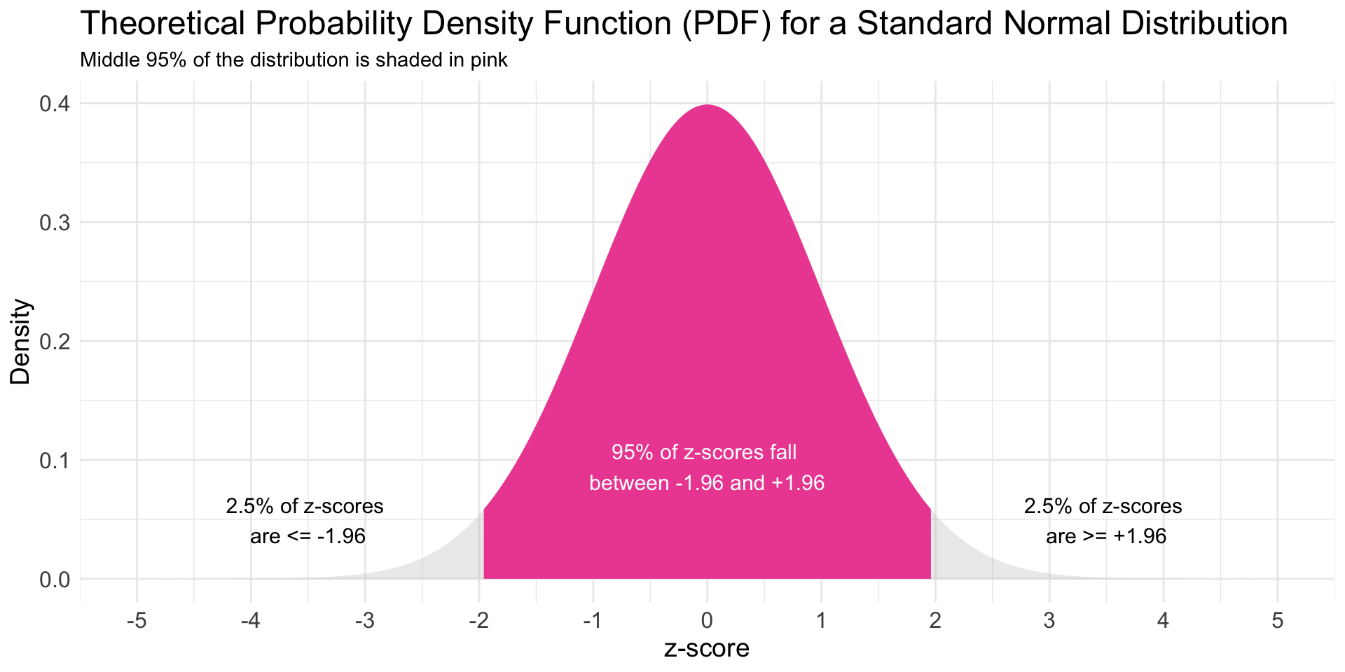
Graph of a Standard Normal Distribution: Middle 95% shaded
![A graph of a standard normal distribution with mean = 0 and sd = 1 and middle 95% marked]()
95% of a normal distribution falls within 1.96 standard deviations of the mean. A z-score of −1.96 means the value is 1.96 standard deviations below the mean. A z-score +1.96 means the value is 1.96 standard deviations above the mean.
Summary for the Standard Normal Distribution
![A graph of a standard normal distribution with the middle 95% marked]()
Think of the standard normal distribution as a measuring stick for uncertainty. It shows what outcomes are typical (middle ~95%) and what are unlikely — and powers confidence intervals, margins of error, and significance tests.