From Question to First Figure
Lecture · Module 3 · Mon Aug 31
Last week, this week
Last week, we worked on the sentence: what am I trying to learn?
Today, we work on the shape: what would evidence for that question look like?
Along the way we learn two things: why a careful plot is not optional, and how to build a figure that helps a reader see the point.
Today’s class has five phases:
- Datasaurus Dozen — a hands-on discovery that settles why we plot at all.
- Chart anatomy — take apart a published chart using grammar-of-graphics vocabulary.
- Chart quality — use Cairo’s five qualities to decide what makes a chart effective.
- Communication moves — turn a competent plot into a figure with a clear point.
- Question-to-Figure Studio — sketch the first chart that could answer your own Week 1 research question.
Why plot at all?
Everything else today — what makes a chart good, how to build a good one — assumes you have accepted that you must make one. So we start there.
The temptation, especially as the statistical machinery gets more sophisticated, is to skip the picture and go straight to the numbers. The next fifteen minutes exist to argue otherwise — and you will be the one making the discovery, with your partner.
The setup: an R package called datasauRus ships 13 different datasets in one tibble called datasaurus_dozen. Each dataset has two variables, \(x\) and \(y\), and the same number of observations. Here’s a peek at the structure:
You should see 13 dataset names: dino, away, h_lines, v_lines, x_shape, star, high_lines, dots, circle, bullseye, slant_up, slant_down, and wide_lines.
Activity 1 · compute summary statistics for one dataset
In the chunk below, change "dino" to any of the 13 dataset names, then click Run Code:
Every dataset has essentially the same five summary statistics: mean(x) ≈ 54.27, sd(x) ≈ 16.77, mean(y) ≈ 47.83, sd(y) ≈ 26.94, and corr(x, y) ≈ -0.06. To two decimal places, they are identical. If you used only the summary numbers to write up these datasets, you would describe all 13 in the same paragraph.
Activity 2 · plot the dataset you picked
So the summary statistics are the same. What about the data themselves?
Now run the chunk. Use the same dataset name you picked above:
The plots look completely different from each other, even though the summary statistics are identical.
Several contain strong structures with a correlation near zero, because Pearson’s correlation only measures the linear part of a relationship. It is not lying to you; it is answering a narrower question than the one your eyes are asking.
Finish this sentence with your partner:
The same numerical summaries can hide _____.
The reveal — all 13 at once
The lesson, written out
If you only inspect summary statistics, you will be wrong about your data — sometimes spectacularly wrong. The Datasaurus Dozen is engineered to make the point, but real data do this all the time, just less theatrically.
Modes, gaps, ceiling effects, bimodality, censoring, recording errors, single-value dominance — every one of these can be invisible at the level of the summary statistics. The truly reliable way to see them is to plot.
So the first move of every analysis you do this semester is: load the data, look at the structure, plot it.
Taking apart a chart in the wild
So plotting is not optional. The next question is what a serious plot is actually made of.
On Friday, you built a Rosling-style chart one layer at a time. You now know enough to read someone else’s chart the same way: data, aesthetic mappings, geoms, scales, labels, and theme choices.
The chart below was made by a professional data-visualization designer, published, and shared with its source code. Before we talk about what makes a chart good, we are going to take this one apart and name its pieces.
Where this chart comes from
TidyTuesday is a weekly social data project run by the Data Science Learning Community. Every Tuesday a new dataset is posted, and people around the world build something from it and share both the chart and the code that made it.
The dataset behind this chart is from Opportunity Insights — anonymized tax records linking where students came from economically to where they ended up. You will meet related college-mobility data again in M07 and M08.

Graphic by Nicola Rennie, reproduced under CC BY 4.0. Data: Opportunity Insights.
| Layer | In this chart | The code idea |
|---|---|---|
| Data | One row per college × parent-income band | plot_data |> ggplot() |
| Aesthetics | x = attendance/application ratio; y = parent income band; color = school group |
aes(x = ..., y = ..., color = ...) |
| Geometry | One dot per college, nudged sideways so overlapping dots stay visible | geom_beeswarm() |
| Facets | Not used | one panel |
| Statistics | Not used | raw observed values, not averages or model fits |
| Scales | Income bands reversed; colors chosen deliberately | scale_y_discrete(limits = rev), scale_color_manual() |
| Labels / theme | Title, subtitle, caption, minimal theme, legend switched off | labs(), theme() |
Two footnotes to give more context:
The data layer is the hand-off, not the cleaning. plot_data did not arrive in that shape. Rennie built it first — selecting three columns, dropping missing rows, and collapsing six school types into three — and only then handed the result to ggplot(). That wrangling is real work, and it is M04’s subject, but it is not part of the grammar. The grammar starts the moment a tidy data frame is piped into ggplot().
geom_beeswarm() is geom_point() with a rule about overlaps. Underneath, it draws points and applies a position adjustment that shifts overlapping ones sideways until each is visible, rather than letting them pile up on the same spot. With several hundred colleges in every income band, plain geom_point() would render a solid stripe and hide exactly the spread the chart exists to show. Worth knowing when your own scatter turns into a blob. geom_jitter() does a similar job, and it’s part of ggplot2. geom_beeswarm() must be installed separately.
What the x-axis actually measures
For today, read the x-axis this way:
Are students from this parent-income band attending this college more or less often than their application rate would suggest?
- A value near 1 means attendance is roughly in line with application.
- A value below 1 means they appear less often among attendees than their application rate would suggest.
- A value above 1 means they appear more often.
That is enough to see the main pattern: the dots spread much wider at the top of the parent-income distribution than at the bottom.
It is also an awkward quantity, and it is not a simple acceptance rate. A high value could reflect admissions decisions, enrollment decisions after admission, or both.
So one fair reading of this chart is:
Students from the highest-income families appear to attend some colleges more often than their application rates alone would suggest, and this pattern is especially variable at the very top of the income distribution.
That is more precise than saying:
Students from the highest-income families have higher college acceptance rates.
The useful lesson is not that the chart is bad. It is very good. The useful lesson is that beautiful design does not remove the need for precise claims.
What makes a chart effective?
Two things are now settled: you have to plot, and a plot is made of nameable parts. That leads us to the next question: once you have plotted, what makes one chart good and another bad?
Let’s consider two design vocabularies that answer that question from different angles:
- Dr. Alberto Cairo’s five qualities help you diagnose whether a finished chart is doing its job.
- Cole Nussbaumer Knaflic’s design moves help you produce a chart that does its job in the first place.
Cairo tells you what to check. Nussbaumer Knaflic tells you what to do.
Cairo’s five qualities
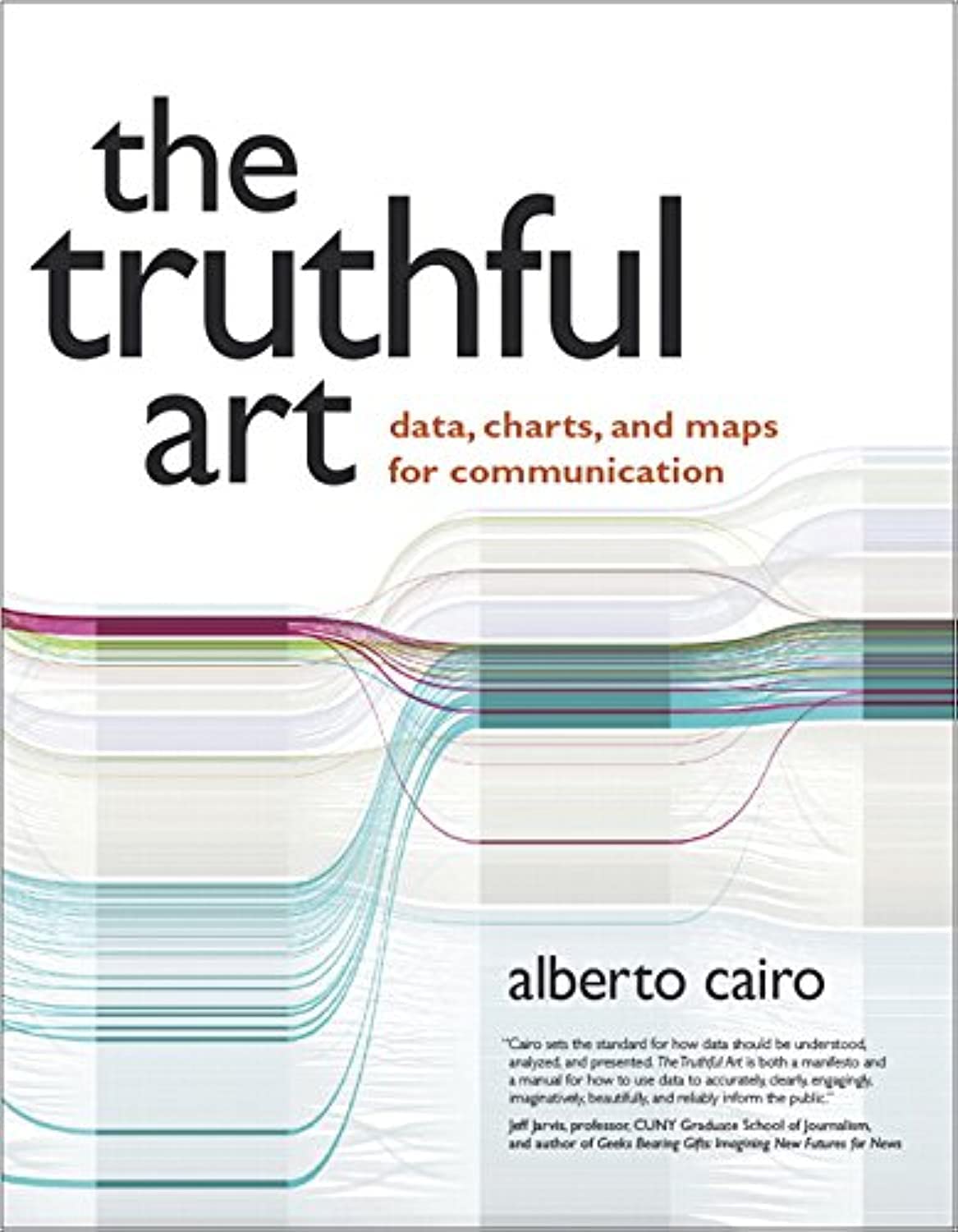
Alberto Cairo proposes that an effective visualization should be all five of the following:
- Truthful — based on thorough, honest research. No misleading axes, no cherry-picking, no visual tricks that do not reflect the data.
- Functional — an accurate depiction of the data that lets the reader do meaningful operations on it.
- Beautiful — attractive and appropriate for the intended audience.
- Insightful — reveals evidence that would be hard or impossible to see in raw numbers.
- Enlightening — changes how the reader thinks about the question at hand.
A chart that is truthful, functional, and beautiful — but not insightful — is still a missed opportunity. A chart that is insightful, enlightening, and beautiful — but not truthful — is worse than a failure; it is a lie.
Score two charts (3 min each)
I am going to put two charts on the screen. Both plot the same data.
They are deliberately not printed here — score them from the screen as we go, then we’ll compare readings as a group.
Fill this in on your own first, before we discuss.
| Quality | Chart A | Chart B |
|---|---|---|
| Truthful | ||
| Functional | ||
| Beautiful | ||
| Insightful | ||
| Enlightening |
Nussbaumer Knaflic’s design moves
Cairo gave us a scorecard. Nussbaumer Knaflic gives us a sequence — six moves that take a chart from “it plots” to “it communicates.”
The six moves
- Understand the context — who’s reading, what do they already know, what action do you want them to take?
- Choose an appropriate display — line, bar, scatter, table; the choice flows from the question, not from your tools.
- Eliminate clutter — every pixel that isn’t carrying meaning is working against the chart.
- Focus attention — color, size, and contrast direct the eye to the finding.
- Think like a designer — alignment, whitespace, and a clear hierarchy of type (what should the reader notice first, second, third? — size, weight, and color set that order, so the title outranks the axis labels, which outrank the gridlines).
- Tell a story — title as finding, annotation as narration, caption that situates.
The first two happen before you write any ggplot: understand the context is the audience-and-action question you answer when you decide why you’re making the chart, and choose an appropriate display is the line-vs-bar-vs-scatter decision that follows from the research question. The tabs below do everything from move 3 onward.
One chart, five versions
Before any code, the question. We want to know whether the United States stands apart from comparable countries in after-tax income inequality — and whether it does so across the whole period, or only recently. Our reader is a room of researchers, and the action we want is that they leave able to state that comparison correctly, including its limits.
That is a question about a quantity moving over time across a handful of groups, which is what points us to a line chart rather than bars or a table.
And one more decision before any code: who is in the chart? “Comparable countries” has to mean something specific, and we have to fix it now — because deciding after we have seen the lines is how cherry-picking happens, usually without anyone intending it. So, we’ll choose the G7. A group defined by someone else, for reasons unrelated to inequality, that a reader can verify and we cannot quietly adjust. The United States is in it by definition rather than by our choosing.
That is the same discipline as writing down your analysis plan before collecting data, and it costs one sentence.
Those three paragraphs were moves 1 and 2, done before opening R. Everything in the tabs below is moves 3 through 6.
inequality_tidy · 7 countries · 34 years · TidyTuesday 2025-08-05
| Variable | Type | What it is |
|---|---|---|
| country | text | One of 7: United States, United Kingdom, Germany, France, Italy, Canada, Japan |
| year | numeric | 1990–2023 |
| gini_dhi | numeric | Gini coefficient of equivalized disposable household income — after taxes and most benefits. Higher = more unequal. |
Source: TidyTuesday, 2025-08-05, from the Luxembourg Income Study.
Coverage is uneven, and we are not hiding it. Italy and Japan report far fewer years than the rest (Japan’s series does not start until 2008), so only 6 of the 34 years have all 7 countries reporting. Short, ragged lines are the honest cost of following a rule instead of picking whichever countries drew nicely. It is also why the final chart labels each line with its own last year, and why its title claims only what the coverage supports: highest in every year a peer also reported — true in all 32 such years.
Each tab applies one move on top of the previous tab’s code. Click through in order — the changes from tab to tab are the moves.
A bare-bones ggplot() — three lines of code, all 7 series on screen. It is a perfectly good exploratory chart: you can see the broad pattern, spot the outlier, and check that nothing looks broken. What it is not is designed for a particular reader or a particular takeaway. That’s the gap the next four tabs close.
The gray panel and the minor gridlines aren’t carrying meaning — they’re just noise. Drop them. Same data, same lines; less for the eye to filter.
Seven equally-weighted colors give the eye nowhere to land — not because seven is too many in principle, but because nothing in the design says which comparison carries the story. Our takeaway is about the United States, so we color that series and mute the rest. The design choice follows from the purpose, not from a rule about line counts.
Notice what the previous tab cost us: suppressing the legend told the reader which line matters, but it also left the gray lines unidentified. Rather than restore a separate key — which would force readers to bounce between chart and legend, and would give equal billing to every series — put each country’s name directly at the end of its own line.
This is the move you already met on the opening chart today, where the designer put the three group names, in their own colors, inside the subtitle.
The last move pulls everything together: a title that states the finding, a subtitle that names what’s measured, a source caption, and one annotation inside the chart that narrates the takeaway. This is the chart that goes in a research talk.
The annotation layer · why the last move is the editorial one
A useful reframe from Michela Tjan at the Open Visualization Academy: every chart has two layers. The data layer shows what happened. The annotation layer — title, labels, the sentence written on the plot — says what it means.
One is description; the other is argument. Tabs 1–4 improve the data layer. Tab 5 adds the argument, and it is the only layer a reader can act on.
Question-to-Figure Studio
Cairo and Nussbaumer Knaflic matter most when they help you communicate something you want to understand. So we are going back to the question you already wrote.
Last Monday, you posed a research question, named its type of inquiry, specified a population, and said how you would measure your variables. Have that Week 1 discussion post or question card open. For the next 20 minutes you are going to do the next thing a researcher does with a question: draw the figure that would answer it.
This is not a results figure — you have no data. But you will have to imagine a result in order to draw anything, and that is the point. Sketching the answer you expect forces you to decide, in advance, what an answer would even look like. Questions that cannot survive that step are usually not yet answerable.
Reader test
Wrap-up · three things to carry into the lab
Three principles, and what comes next
- Never let a summary stand in for a careful look. The Datasaurus rule. Means, SDs, and correlations are real information — they are just incomplete, and what they omit is exactly what a plot shows.
- Chart design is editorial. Every encoding decision is a small choice about what to emphasize and what to fade.
- For communication charts, make the takeaway easy to find. A supported, finding-oriented title is the simplest way to do it — written after you have checked that the claim holds.
Wednesday’s lab puts all of this into practice on your own machine. You will import data, build a plot, critique it with Cairo’s five qualities, and revise it. That is the full loop for the first time: question, data, figure, critique, revision.