Writing with Code

Inline R, cross-references, and citations — the quick reference for project reports

For your project reports, anything derived from your data must be generated by code, not typed. Numbers in prose come from inline R. “Figure 1” and “Table 1” come from cross-references. For Project 2, the References section comes from a .bib file. You will practice each piece in a lab — inline R and figure references in the M04 lab, citations in the M08 lab — and this page collects all of the syntax in one place so you don’t have to dig back through them mid-project.

See it inside a real notebook

This page has to escape the inline-R syntax to display it. The companion notebook doesn’t: writing-with-code-demo.zip contains a runnable .qmd (plus a mini references.bib) using every technique below for real. Extract it anywhere, open the .qmd in RStudio, click Render, then read the source and the rendered HTML side by side. It ends with three “break it on purpose” exercises that show you common hiccups.

A tiny dataset to demonstrate with

Every example below runs live on this page, using a twelve-person toy dataset defined right here — so what you see rendered is what the syntax actually produces:

demo_survey <- tibble(
  respondent  = 1:12,
  use_group   = rep(c("Uses daily", "Less often"), times = c(7, 5)),
  hours_online = c(4.5, 3.0, 5.5, 4.0, 6.0, 3.5, 5.0,
                   1.5, 2.0, 1.0, 2.5, 1.5)
)

demo_survey |> count(use_group)

Inline R

The two-step pattern

Step one — compute the number and give it a name, in a chunk:

```{r}
#| label: headline-numbers

n_total   <- nrow(demo_survey)
pct_daily <- demo_survey |>
  summarize(p = mean(use_group == "Uses daily") * 100) |>
  pull(p)
hours_gap <- demo_survey |>
  group_by(use_group) |>
  summarize(m = mean(hours_online)) |>
  pivot_wider(names_from = use_group, values_from = m) |>
  mutate(gap = `Uses daily` - `Less often`) |>
  pull(gap)
```

Step two — call the name in your sentence. In your prose (not in a chunk), type:

Of the `r n_total` respondents, `r round(pct_daily, 1)`% use social
media daily, and daily users spent `r round(hours_gap, 1)` more hours
online per day on average.

That exact markdown renders as:

Of the 12 respondents, 58.3% use social media daily, and daily users spent 2.8 more hours online per day on average.

Change the data and/or analysis, re-render, and every number in the sentence updates itself. A typed digit is correct only until the next time your team revises the wrangling — and nothing warns you when it stops being true. Inline R makes prose-vs-table disagreement impossible, because both are computed from the same object.

The syntax is exactly: backtick, the letter r, a space, an R expression, backtick. No curly braces (those belong to chunks), no quotes.

The single-number rule

The object you call inline needs to hold one value — not a data frame. The pull() function extracts a single column from a data frame or tibble, and if you filter to one row first, you get a single value. The example below shows both the wrong way (a 1-row, 2-column tibble) and the right way (a single number).

```{r}
#| label: single-number-trap

# NOT yet inline-ready -- this is a 1-row, 2-column tibble:
demo_survey |>
  group_by(use_group) |>
  summarize(m = mean(hours_online)) |>
  filter(use_group == "Uses daily")

# Inline-ready -- pull() extracts the single value:
daily_mean <- demo_survey |>
  group_by(use_group) |>
  summarize(m = mean(hours_online)) |>
  filter(use_group == "Uses daily") |>
  pull(m)

daily_mean
```

[1] 4.5

The habit: end the pipeline with pull(), and print the object once in the chunk so you can see what you got before using it via inline R for prose.

Formatting the value

Wrap the inline call in a formatting function so the rendered number reads like prose, not like console output:

Formatting helpers for inline values

You want	Type inline	Renders as
Fewer decimals	r round(daily_mean, 1)	4.5
Big numbers with commas	r scales::comma(1502187)	1,502,187
A percentage from a proportion	r round(0.3842 * 100, 1)%	38.4%

The chunk that defines an object to be used inline must appear above the sentence that calls it: Quarto evaluates the document top to bottom.

Cross-referencing figures

Three ingredients make a chart citable as “Figure 1”: a chunk label starting with fig-, a fig-cap, and the @ reference in your prose.

```{r}
#| label: fig-hours-by-group
#| fig-cap: "Hours online per day by social-media use group."

demo_survey |>
  ggplot(aes(x = use_group, y = hours_online)) +
  geom_point(size = 3, alpha = 0.7, color = "#4E5EAA") +
  labs(x = NULL, y = "Hours online per day") +
  theme_minimal(base_size = 13)
```

Then in your prose, type @fig-hours-by-group — plain text, no backticks around it. This sentence does exactly that: as Figure 1 shows, daily users cluster well above the others.

demo_survey |>
  ggplot(aes(x = use_group, y = hours_online)) +
  geom_point(size = 3, alpha = 0.7, color = "#4E5EAA") +
  labs(x = NULL, y = "Hours online per day") +
  theme_minimal(base_size = 13)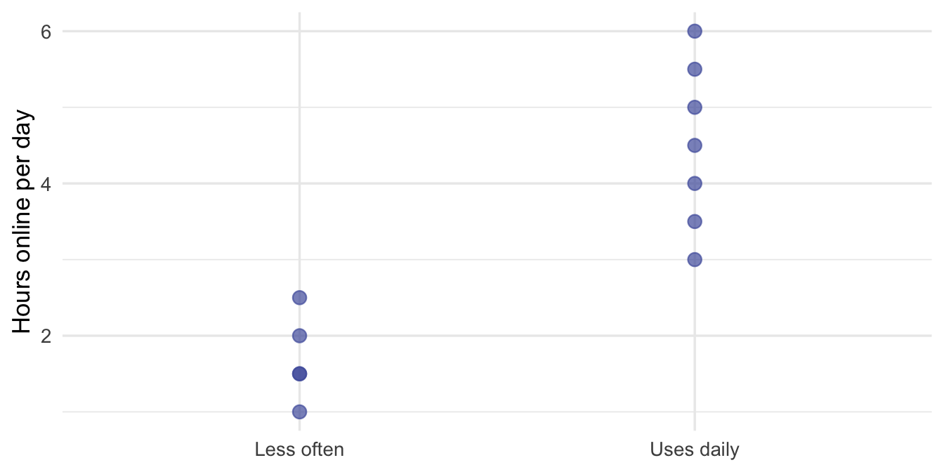

Figure 1: Hours online per day by social-media use group.

Notice what happened in the rendered page: the caption gained a figure number automatically, the @fig- reference became the clickable text “Figure 1,” and the numbering follows the order figures appear in the document — reorder your sections and the numbers renumber themselves.

The rules, compactly:

• The label must start with fig-; use hyphens in the rest of the name, not underscores or spaces.
• No caption, no number — a fig-cap is what turns the chunk output into a numbered, referenceable figure.
• Reference it as @fig-name in plain prose.
• After rendering, click every figure link to confirm it jumps where you expect.

Cross-referencing tables

Tables work the same way with tbl- in place of fig-: label the chunk tbl-something, give it a tbl-cap, reference it as @tbl-something.

```{r}
#| label: tbl-group-summary
#| tbl-cap: "Hours online per day, summarized by use group."

demo_survey |>
  group_by(use_group) |>
  summarize(n = n(), mean_hours = round(mean(hours_online), 1)) |>
  knitr::kable()
```

In prose: @tbl-group-summary — and Table 1 below shows the result.

demo_survey |>
  group_by(use_group) |>
  summarize(n = n(), mean_hours = round(mean(hours_online), 1)) |>
  knitr::kable()

Table 1: Hours online per day, summarized by use group.

use_group	n	mean_hours
Less often	5	1.7
Uses daily	7	4.5

This works identically when the chunk’s output is a gtsummary::tbl_summary() or a gt() table — which is exactly how your Project 1 Table 1 becomes citable: for example, label its chunk tbl-one, caption it, and write @tbl-one in the prose that walks the reader through it.

Citations from references.bib

You don’t need to include references for Project 1, but you will for Project 2. The M08 lab demonstrates this technique. This page provides a compact example.

There is no need to type an APA reference by hand. Entries live in your project’s documentation/references.bib, and Quarto builds the citation and the References section from them.

A .bib entry looks like this:

@article{hofman2020,
  author  = {Hofman, Jake M. and Goldstein, Daniel G. and Hullman, Jessica},
  title   = {How visualizing inferential uncertainty can mislead readers
             about treatment effects in scientific results},
  journal = {Proceedings of the 2020 CHI Conference},
  year    = {2020},
  doi     = {10.1145/3313831.3376454}
}

The part after the { on the first line — hofman2020 — is the citation key. In your prose:

The two citation forms

You type	Renders as	Use when
[@hofman2020]	(Hofman et al., 2020)	Parenthetical — the claim is yours, the source supports it
@hofman2020	Hofman et al. (2020)	Narrative — the authors are the subject of your sentence

(The exact punctuation follows the citation style. The Project 2 starter pins APA 7 with a csl: apa.csl line in its YAML — the same styling your M08 paper got automatically from its apaquarto format — so you get the forms shown above. In a document with no csl: line, Quarto’s default author–date style renders “(Hofman et al. 2020)” — same machinery, different styling.)

The smooth workflow, from the M08 lab: in RStudio’s Visual editor, Insert ▸ Citation… opens a dialog that can look a source up by DOI, write the .bib entry for you, and insert the key — no hand-typed BibTeX at all. The References section then assembles itself at the end of the rendered document, formatted by the CSL style, containing exactly the sources you cited.

One wiring note: the Project 2 starter is fully set up — its YAML already points at the shared bibliography (bibliography: ../documentation/references.bib) and pins the APA reference style (csl: apa.csl, shipped in programs/). There is nothing to install or configure; just add entries and cite.