Revenge, Two Weeks Later
Lecture · Module 10 · Mon Nov 2
How today works
The M10 Module fit three regressions on benevolence in the REACH trial. Today we fit the same three on a different outcome from the same questionnaire: revenge. Same data, same code, new answers. That gives you a second pass through everything the Module covered. A Going further section at the end runs the Module’s regression toward the mean on revenge, using it to catch a mistake applied researchers make often.
Today’s plan
| Part | The question | The Module section it revisits |
|---|---|---|
| Meet revenge | Where do people start? | The REACH study and its measures |
| Part 1 | Does revenge now predict revenge two weeks later? | Part 1: a continuous predictor (the line, centering, R² and \(\sigma\), inference, CI vs PI) |
| Part 2 | Did the workbook reduce revenge? | Part 2: a binary predictor (the slope as a mean difference, the t-test, Cohen’s d) |
| Part 3 | Does revenge differ across the six sites? | Part 3: a categorical predictor (dummies, the reference group, the omnibus F) |
Meet revenge
REACH’s questionnaire, the TRIM-18, has three subscales. The Module used benevolence (goodwill toward the person who hurt you). Today’s outcome is revenge: five items such as “I’ll make him or her pay” and “I want to see him or her hurt and miserable,” each rated from 1 (strongly disagree) to 5 (strongly agree). Each person’s score is the average of the five, so it runs from 1 to 5, and higher means more revenge. The file we’ll work with today has it twice: t1_revenge at baseline and t2_revenge two weeks later.
Pair-and-share · predict first
Benevolence scores sat near the middle of the 1–5 scale, spread fairly evenly around it. Where do you think baseline revenge scores sit? In the middle too, or piled up near one end? Sketch the histogram you expect, then open the answer.
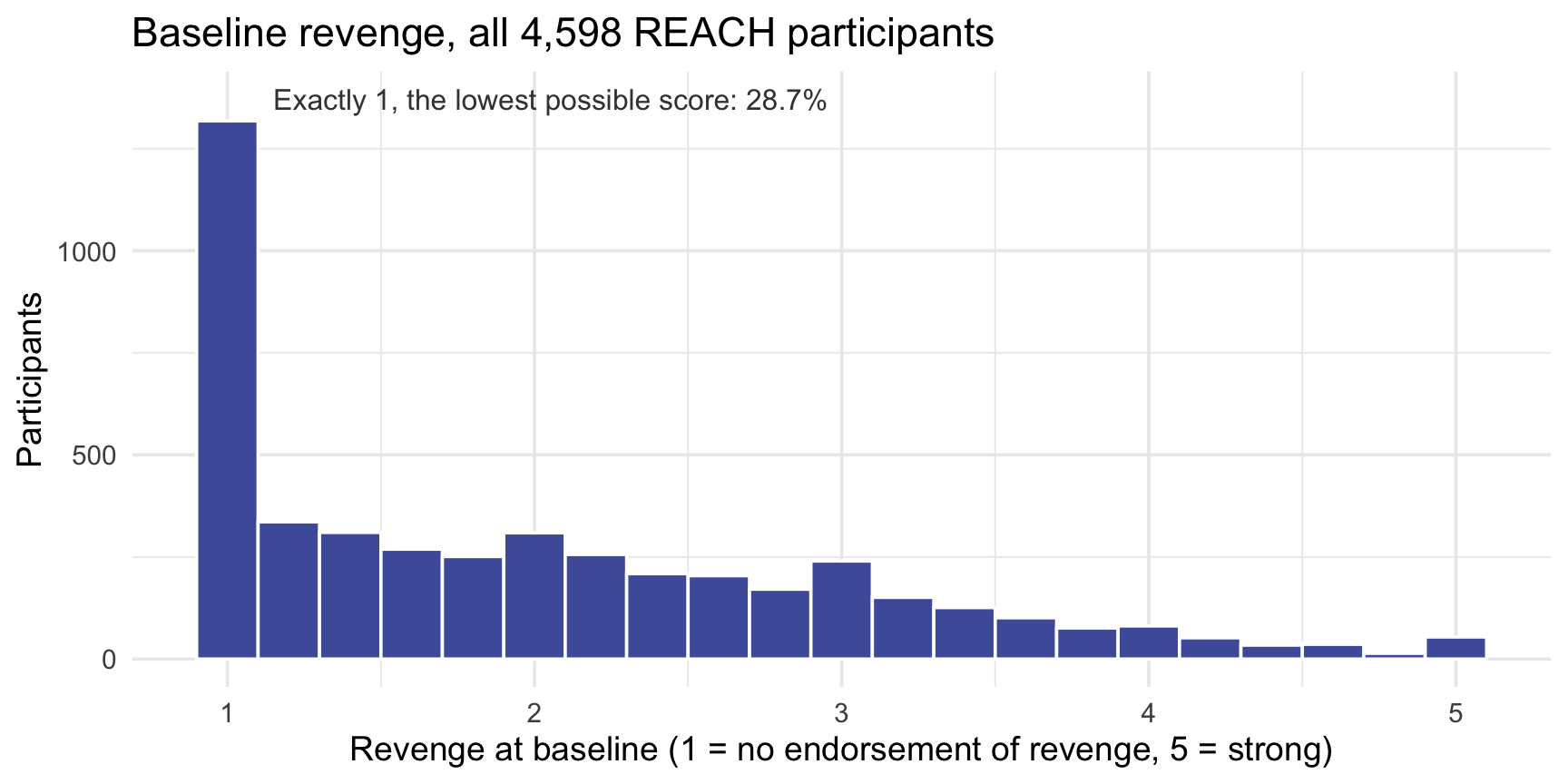
Piled up at the bottom. Nearly 3 in 10 participants (28.7%) gave the lowest possible answer, 1, on every item, and the rest trail off to the right (mean 2.00, SD 1.02). Most people who are dealing with a hurt don’t endorse wanting revenge, and the scale can’t go below 1 to show how much they don’t. Statisticians call a pile-up at the lowest possible value a floor effect. Keep it in mind: it matters at the end of today, and again in M12, when we check the model’s assumptions.
Part 1 · Does revenge now predict revenge two weeks later?
As in the Module’s Part 1, we start with Hong Kong’s waitlist arm: 173 people who completed both questionnaires and had no workbook during the two weeks. A small sample keeps the picture readable, and with no workbook, the question is simply how revenge carries over from one questionnaire to the next, two weeks later.
Plot before you fit
The cloud rises from lower left to upper right, and a straight line is a reasonable summary of it. Notice the few people at a baseline of 1: they can’t score any lower, at either time.
Fit the line and read it
Read the output · six questions
Answer each from your output before you open the answers.
- What does the slope say, in one sentence about people?
- What does the intercept say, and is it a useful number here?
- What do R² and \(\sigma\) say?
- What do the slope’s 95% CI and its test say?
- What does the F-test in glance() test, and how does it relate to question 4?
- Your guess from the pair-and-share: steeper, flatter, or the same as benevolence’s?
- Slope, 0.597. Comparing two people in this arm whose baseline revenge differs by 1 point, the one with the higher baseline is predicted to score about 0.60 points higher two weeks later. It’s a comparison between people, not a statement about one person’s change.
- Intercept, 0.994. It’s the predicted follow-up score for a baseline of 0, and the scale starts at 1, so no one can have that baseline: it locates the line but isn’t worth interpreting. Centering fixes that, as in the Module: subtract the mean baseline (2.82) from everyone’s score and refit, and the intercept becomes 2.68, the predicted follow-up score for someone at the average baseline, which is exactly the arm’s average follow-up score. The slope doesn’t change.
- R² = .450: baseline revenge accounts for about 45% of the variation in follow-up revenge. (In a simple regression, R² is the correlation squared: r = .671, and .671² = .450.) \(\sigma\) = 0.645, the residual standard error: the model’s estimate of the SD of the errors, the typical scale of the scatter around the line, in revenge points. In revenge terms: even knowing someone’s baseline, our prediction of their follow-up revenge is typically off by something on the order of 0.64 of a point on the 1-to-5 scale, so for someone predicted at 2.5, a follow-up score anywhere from about 1.9 to 3.1 would be unremarkable. Compare it with the follow-up scores’ own SD, 0.867: knowing someone’s baseline shrinks the spread of our misses from 0.87 to 0.64. To picture it, use the empirical rule: if the errors are roughly Normal, about 68% of people (roughly two-thirds) land within ±1\(\sigma\) of the line, and about 95% within ±2\(\sigma\). Here 73% and 95% do.
- 95% CI [0.497, 0.696], with \(t_\text{obs}\) = 11.8 on 171 degrees of freedom and p < .001. The slope’s SE, 0.050, is the sample-to-sample wobble the Module’s bootstrap made visible. The test of a zero slope isn’t very informative here: no one expected revenge two weeks apart to be unrelated. The CI is the more useful part: it rules out slopes near 0 and slopes near 1.
- F(1, 171) = 140.1, p < .001. The F-test asks whether the model as a whole accounts for more of the variation in follow-up revenge than chance alone would: the variance the line explains, per df, divided by the leftover variance, per df (the Module’s MSR / MSE). Its df are 1 (one slope) and n − 2 = 171. With a single predictor, “does the model explain anything?” and “is the slope different from 0?” are the same question, so it’s the same test as question 4: F is \(t_\text{obs}\) squared (11.84² ≈ 140.1), and the two p-values are identical. The F-test earns its keep later, when a model has several predictors and we ask whether they help together.
- About the same, a little flatter: 0.60 against benevolence’s 0.62. Both are well below 1. The Going further section at the end looks at what a slope below 1 can mean.
Using the model to predict
What follow-up score should we expect for someone who starts at a baseline revenge of 4?
Start with the equation. The fitted line is \(\hat{y} = b_0 + b_1 x\). Plug in the intercept and slope from tidy() and a baseline of 4:
\[\hat{y} \;=\; 0.994 + 0.597 \times 4 \;=\; 3.38\]
So the model predicts a follow-up revenge score of about 3.38 for anyone who starts at 4. The residual is how far a real person lands from that prediction: observed minus predicted, \(e = y - \hat{y}\). Suppose a client who started at 4 reports a 3 two weeks later. Her residual is 3 − 3.38 = −0.38: she sits 0.38 points below the line, a little less vengeful than the model predicted. A positive residual would put her above it.

predict() does the same arithmetic for you. Give it a small data frame holding the baseline score you want, with the same column name the model uses, and it returns \(\hat{y}\):
Same 3.38 as the equation gave.
Uncertainty for predictions: one person, or the average person?
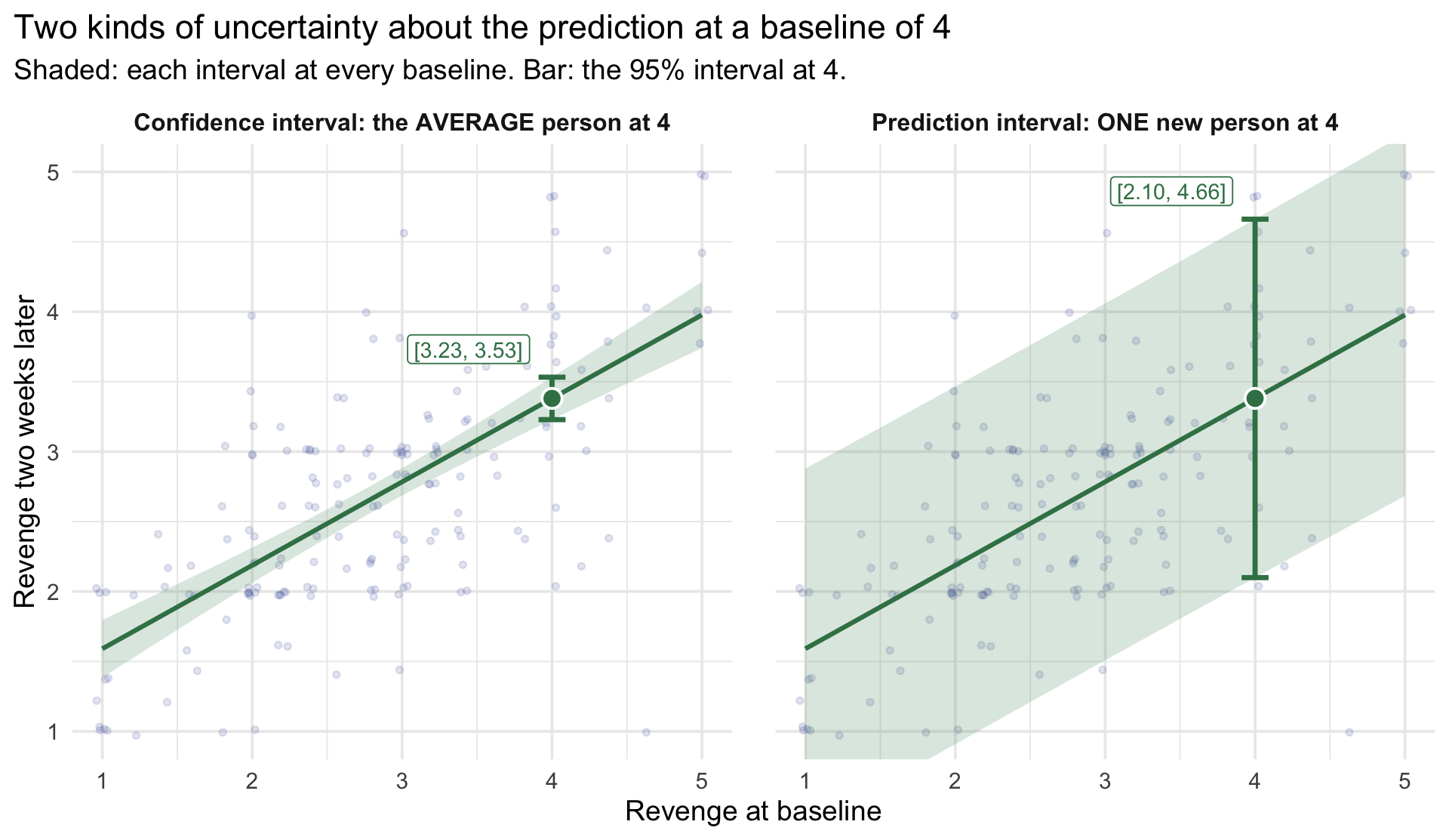
That 3.38 is a single best guess, and like every estimate from a sample, it comes with uncertainty. The question “what follow-up score should we expect at a baseline of 4?” has two versions, and they carry different amounts of it:
- The average follow-up score among everyone who starts at 4. The only uncertainty is where the line itself sits: a different sample of 173 people would have given a slightly different line. A confidence interval captures that.
- One new person’s follow-up score at 4. That uncertainty includes where the line sits, plus the person-to-person scatter around it, the \(\sigma\) from earlier. A prediction interval captures both.
Add interval = to predict() to get each one:
Here are both, drawn on the same picture as before. The shading shows each interval at every baseline; the bar is the interval at 4.
Part 2 · Did the workbook reduce revenge?
Now the question REACH was built to answer, with revenge as the outcome. As in the Module’s Part 2, we use everyone with a follow-up score, in both arms: 2,057 on the waitlist and 1,907 who got the workbook. The predictor is the factor treat; lm() codes it as 0 for the waitlist (Control) and 1 for the workbook (Treatment).
The picture. The regression line just connects the two arms’ means. Moving from the waitlist to the workbook is a run of 1 on the 0/1 predictor, and the rise over that run is the slope. The faint dots show how much the two arms overlap, even though their means clearly differ; Cohen’s d below puts a number on that.

The same comparison, two ways. A regression with a binary predictor and the standard (equal-variance) two-sample t-test are the same model. Check it:
The statistic matches the regression’s \(t_\text{obs}\) (−13.07), and the interval matches its CI. How big is the effect? Cohen’s d is the difference in SD units: the slope divided by \(\sigma\) from glance(), −0.359 / 0.865 = −0.42. By Cohen’s rough benchmarks, that falls between a small (0.2) and a medium (0.5) effect.
Part 3 · Does revenge differ across the six sites?
The Module’s Part 3 compared baseline benevolence across REACH’s six sites. Do the same with baseline revenge, using everyone in the trial:
The picture. Colombia’s mean is the intercept, the dashed line. Each other site’s coefficient is the height of its stick: how far that site’s mean sits above Colombia’s. The faint dots are the R² story: people within any one site range across most of the scale, so knowing someone’s site tells you little about their revenge.

TipGoing further — a common trap: attributing substantive meaning to regression toward the mean
The M10 Module’s section on regression toward the mean, run on REACH’s revenge data. Work through it on your own if you like.
Now imagine REACH had been a different study, with the same people but one arm: everyone gets the workbook, and there is no waitlist. A researcher wants to show that the workbook helps the people who need it most, the ones consumed by revenge, so he analyzes only the most vengeful: those with baseline revenge of 3 or higher (about 1 in 5 people, 21.0%). He compares their revenge before the workbook with their revenge two weeks later. It’s a single-arm study: one group, measured before and after.
REACH’s workbook arm lets us run his study with real people: its 403 most vengeful participants who completed both questionnaires.
Run his study. The chunk keeps REACH’s most vengeful workbook participants and tests their average change against zero with t_test(), the one-sample test from M08.
What would he conclude?
His most vengeful group’s revenge fell by 1.50 points on a 1-to-5 scale, \(t_\text{obs}\)(402) = −29.6, p < .001. What would he write in his abstract? What would a reader conclude about the workbook?
But REACH had a waitlist. 431 of REACH’s most vengeful people didn’t get the workbook during those two weeks. Run the same analysis on them:
These people received nothing
The waitlist’s most vengeful group fell by 0.74 points, \(t_\text{obs}\)(430) = −16.5, p < .001: a large, statistically significant “improvement” among people who got no workbook at all. Take a minute with your neighbor: what does that mean for his result?
Why did people who got nothing improve?
Here is every waitlist participant who completed both questionnaires (2,057 people). Two lines help read the picture. The dashed line is where people would sit if each person’s revenge stayed exactly the same. The regression line is the one you’d fit to these points.
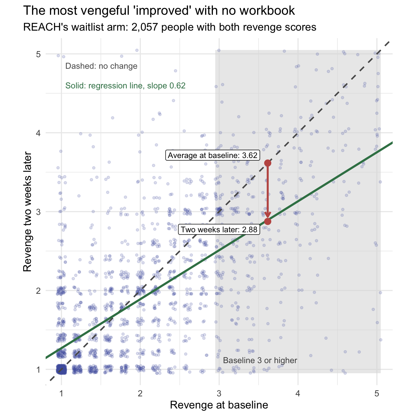
The regression line is flatter than the no-change line: its slope is 0.62, not 1, the same pattern you met in Part 1. A raw slope is the correlation times the ratio of the two SDs, so two things flatten it. Most of the flattening here comes from the imperfect correlation between the two occasions (r = .67); a little comes from follow-up scores being less spread out than baseline scores (SD 0.94 against 1.02), with more people at the floor. The correlation part has a name: regression toward the mean. When two measurements are imperfectly correlated, people with extreme scores on the first tend, on average, to be less extreme relative to the second.
Why it happens. Anyone’s revenge score on a given day is part lasting (how they generally feel about the person who hurt them) and part that-day (how raw the hurt felt that week, how they read a question, their mood when they filled it in). People selected for especially high baseline scores tend to have both a genuinely high lasting level of revenge and an unusually high that-day part on that particular occasion. Two weeks later, the lasting part is still there, but the that-day part need not run high again, so on average the group’s scores fall back toward the mean. No one has to change for this to happen. Selecting people because they scored high builds part of the drop in, on average.
The regression line predicts it. For the waitlist’s most vengeful group, average baseline 3.62, the line predicts 0.648 + 0.621 × 3.62 = 2.89 two weeks later. They actually averaged 2.88. The whole waitlist, by comparison, changed by just −0.12: the big drop came from whom he selected, not from the passage of time.
The other direction: did the workbook harm the least vengeful?
Researchers who select their worst-off participants rarely run the same analysis on their best-off ones. Try it: the people who started with no revenge at all, the lowest possible score of 1 on every item.
Their revenge rose by 0.19 points, \(t_\text{obs}\)(546) = 8.54, p < .001. By his logic, the workbook made the least vengeful people more vengeful. No one would write that conclusion, yet it is exactly the same analysis as “the most vengeful were really helped.” Here are both selections, in both arms:
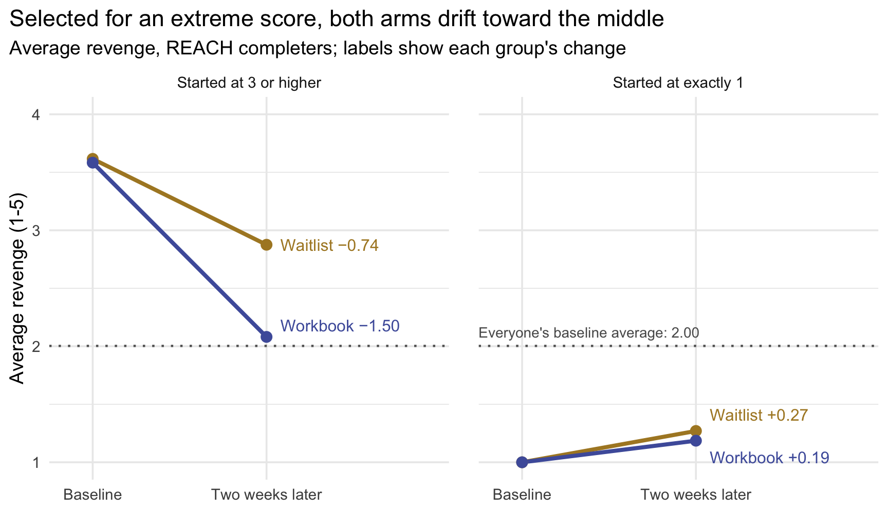
In each selection, both arms move the same way: down for the most vengeful, up for the least vengeful, each back toward the middle. That shared movement is regression toward the mean. (At the floor it can only go one way, because a score of 1 can stay or rise but not fall.) The workbook’s effect is the gap between the arms within each selection: −0.76 among the most vengeful, and only −0.08 among the least vengeful, who had almost no revenge to lose.
The takeaway
Select people because they score extremely, high or low, and, as a group, they will tend to look less extreme next time, with or without your intervention: the worst off will look helped, and the best off will look harmed. A comparison group selected the same way is what tells you how much of the change your intervention caused.
The same applies anywhere people enter a study because a score is high (or low): a clinic that enrolls its most anxious clients, a tutoring program for the lowest scorers on a first exam, a school that flags its most-absent students.
One more: regression toward the mean with no real change at all. You can watch regression toward the mean appear with no real change at all. In this simulation, each person has a lasting level of revenge that stays exactly the same, and each questionnaire adds a little that-day noise. The simulated scores are illustrative and unbounded: unlike the real 1-to-5 scale, they can fall below 1 or above 5. Selecting the top fifth at baseline still produces a drop. Run it, then try a larger or smaller noise and rerun: the more that-day noise there is in each score, the bigger the drop.
Wrapping up
What today covered, with revenge
| The Module’s idea | Today’s revenge result |
|---|---|
| A continuous predictor: plot first, fit, read the slope as a comparison between people | Slope 0.60: two people 1 point apart at baseline are predicted 0.60 points apart two weeks later |
| Centering gives the intercept a meaning | Centered intercept 2.68: the predicted follow-up score at the average baseline |
| R² and \(\sigma\) | R² = .45 (r = .67, squared); \(\sigma\) = 0.645 |
| Inference for the slope | 95% CI [0.50, 0.70]; F = \(t_\text{obs}^2\) |
| CI vs PI | At baseline 4: the average person [3.23, 3.53], one person [2.10, 4.66] |
| A binary predictor: the slope is a mean difference; same model as the t-test | The workbook lowered revenge by 0.36 points; d = −0.42 |
| A categorical predictor: dummies and a reference group | Hong Kong 1.11 points above Colombia; site R² = .095 |
What’s next.
Next Monday, revenge comes back. You’ll put baseline revenge into the model alongside the workbook, the multiple-regression version of today’s comparison, and see how adjusting for where people started sharpens the estimate of what the workbook did.