Revenge, Checked
Lecture · Module 12 · Mon Nov 16
How today works
The M12 Module checked the assumptions behind its model with site, on benevolence. Today we run the same checks on revenge, using the M11 lecture’s model with site (its Part 3), unchanged. Same data, same code as the Module, new answers. Revenge turns out to be a useful second pass, because almost every check comes out as a mirror image of the Module’s.
Today’s plan
| Part | The question | The Module section it revisits |
|---|---|---|
| Opening | Which assumptions matter most? | Part 1: the assumptions, in order of importance |
| Part 1 | Does the model get the average right? | Part 2: linearity; Part 7: additivity |
| Part 2 | Are the errors well-behaved? | Part 3: normality; Part 4: equal variance |
| Part 3 | Is anyone steering the fit? Do the predictors overlap? | Part 5: influence; Part 6: multicollinearity |
| Part 4 | So what do we report? | Part 8: when violations matter |
| After class (optional) | What we didn’t get to in class | Part 8: check_model() and reporting the diagnostics |
The chunk below rebuilds the M11 lecture’s analysis sample and its model with site. The code is identical, down to the names analysis and m2, which is also what the Module calls its model.
Every check today starts from augment(), which adds the model’s per-person results to the data, one row per participant. These are the columns we’ll use:
- .fitted: the model’s prediction for that person.
- .resid: the residual, observed minus predicted (t2_revenge − .fitted).
- .std.resid: the residual divided by its standard error, so every residual is on the same scale.
- .hat: leverage, how unusual the person’s predictor values are.
- .cooksd: Cook’s distance, how much the fit would change without this person.
Opening · “Did you check the assumptions?”
The M11 lecture’s result: participants randomly assigned to the workbook scored an estimated 0.35 points lower on follow-up revenge than those on the waitlist, adjusting for baseline revenge and site, 95% CI [−0.39, −0.31]. You send the draft to a co-author, who replies with one line: “Looks great. Did you check the assumptions?”
Call it out · rank them
Here are six assumptions a regression rests on. Which one would you put first, and which last, for trusting that result?
- Normality of the errors
- Validity: the data map to the research question
- Independence of the errors
- Additivity and linearity
- Representativeness: the sample speaks for the population
- Equal variance of the errors
Regression and Other Stories (ROS, Section 11.1), the book the Module draws on, lists them “in decreasing order of importance”:
- Validity
- Representativeness
- Additivity and linearity
- Independence of errors
- Equal variance of errors
- Normality of errors
The two at the top aren’t about residuals at all: they’re checked with knowledge of the design (what was measured, who was sampled, who is missing), not with a plot. The Module’s Part 1, Two assumptions that come first, works through both for REACH; today we take up the ones the residuals can check. And normality comes last. ROS: “For the purpose of estimating the regression line (as compared to predicting individual data points), the assumption of normality is typically barely important at all.” The acronym LINE (linearity, independence, normality, equal variance) is a memory aid, not a ranking. If your list put normality near the top, you’re in good company: ROS notes that “many textbooks recommend quantile-quantile (Q-Q) plots” for it, yet it’s the one that matters least for a coefficient.
Part 1 · Linearity and additivity: does the model get the average right?
Plot the data with the fitted model first
ROS (Section 11.2) recommends a step before any residual plot: draw the data with the fitted model on top. As in the Module, the model contains site, so each line averages the six sites’ predictions, weighting each site by its number of participants.
The model draws two parallel lines, one per arm, with a gap of 0.35 between them at every baseline. (Today, gap always means the difference between the arms, workbook minus waitlist.) Run the chunk, then look at the far left, at a baseline of 1, where the floor is.
The floor is where the trouble shows. A dense band of people sits along the dashed line at 1: 40% of the analysis sample scored exactly 1 two weeks later. At a baseline of 1, the model’s lines sit at 1.445 (waitlist) and 1.096 (workbook), the same 0.349 apart as everywhere else. The people who actually started at 1 averaged 1.27 and 1.19 two weeks later: a gap between the arms of only 0.08. Most of them hadn’t moved at all: 79% of the workbook arm and 67% of the waitlist were still at 1. And because some sites sit lower than others, 7.9% of the model’s individual predictions are below 1, scores no one can report. Hold on to the gap at the floor: it comes back at the end of this part.
The residual–fitted plot
The edge is along the bottom, slanting down from the left. Someone predicted at 1.1 who reports 1 has a residual of −0.1, and no one can report less than 1, so residuals near the low end of the predictions can’t fall much below zero. In the lowest tenth of the predictions, not one residual is below −0.03. The diagonal stripe running down from the left is everyone who scored exactly 1. It’s the Module’s bounded-outcome wedge, mirrored.
Read the smoother, not the cloud. As the Module says, the wedge is the boundedness story, and the smoother is the linearity story. Here the smoother bends gently. The average residual is 0.19 in the lowest tenth of the predictions, dips to −0.15 in the middle, and rises to 0.10 in the highest tenth.
Is that a linearity problem? Mostly not. Look at who gets the lowest predictions. They’re all workbook participants, and 99% of them started at 1. The model predicts each one’s score by taking the prediction for a similar waitlist participant and subtracting the full 0.35 workbook effect. That puts most of their predictions below 1, a score no one can report. Their actual scores can’t go below 1, so they land above the predictions, and the residuals come out positive. That’s what lifts the left end of the smoother. At the other end, the highest predictions belong mostly to waitlist participants who started high (75%), and the single effect misses them too. That’s the parallel-lines assumption failing, which is additivity, next. When the next section lets the workbook’s effect vary with baseline, the bend nearly disappears: every tenth’s average residual stays within 0.1 of zero. (The Module’s next step, a component-plus-residual plot for each numeric predictor, applies here only to baseline revenge: treatment and site give one mean per group, so they have no line to bend.)
Additivity · is the workbook’s effect the same at every baseline?
The model assumes additivity: the workbook’s effect is the same at every baseline, which is what draws the two lines parallel. A quick look at two groups of people puts that to the test.
Pair-and-share · is the effect the same in both groups?
Split REACH’s completers by where they started. Among people who started at 3 or higher (an average baseline of 3.6), the workbook arm’s revenge fell 0.76 points more than the waitlist’s. Among people who started at exactly 1, the workbook–waitlist gap was −0.08. (The M10 lecture’s Going further section works through both groups.) The additive model gives everyone the same effect, −0.35. Does that allow for both numbers?
No. Checking additivity means fitting a model that lets the workbook’s effect change with baseline revenge, called an interaction model. That’s the core of moderation, which PSY 653 develops, so we won’t fit or interpret it here. Here is what it finds:

The lines stop being parallel. Letting the effect vary, the model implies a workbook effect of −0.08 at a baseline of 1, −0.35 at 2, and −0.61 at 3. At 3.6, the vengeful group’s average, it implies −0.77: both groups’ workbook–waitlist gaps, recovered by a model. (The interaction coefficient is −0.264, 95% CI [−0.306, −0.222]: how much the workbook’s effect changes per point of baseline revenge. PSY 653 develops how to read it.)
Two readings fit this pattern, and a linear model on this scale can’t separate them. One is genuine moderation: the workbook helps most the people consumed by revenge. The other is the floor: someone who reports no revenge has none to lose, so the scale itself caps the effect at 1. The control group doesn’t settle it. Randomization makes −0.08 an honest estimate of the effect on this scale for people who started at 1, but both arms are pinned at the floor, so the comparison can’t show whether the workbook would have done more on a scale that could go lower. This is the Module’s ceiling story, upside down.
So what is the −0.35? Not wrong, but an overall summary: the workbook’s effect at each baseline, averaged over the people REACH enrolled. About 3 in 10 started at the floor, where the effect is near zero, and about 2 in 10 started at 3 or higher, where it averages −0.77.
Part 2 · Normality and equal variance: are the errors well-behaved?
Normality · the histogram and the Q–Q plot
Skewed right (skewness 1.13). Start with the histogram: a tall, narrow pile near zero, mostly people at the floor whose scores sit at or a little below their predictions, and a long tail stretching to the right. The rose curve shows what Normal errors would look like, and the bars miss it in three places. The pile rises far above it: the bar at zero holds 653 people, where a Normal would put about 394. The bars on either side of the pile fall short of it. And the right tail runs on where the curve has gone flat: a Normal would put about 5 people above 3, and revenge has 51. The Q–Q plot shows the same shape as a bend. It lines the residuals up from smallest to largest against where they’d fall if they were Normal, so the histogram’s long right tail becomes the upper end climbing far above the line: people far more vengeful than predicted. The lower end stays close to the line, dipping only a little below it in the last few points. The floor caps how far below zero a residual can fall only where the predictions sit near 1; people predicted higher up can still land well below their predictions, so the lower tail looks roughly Normal. The skew comes from the upper tail.
Where did the histogram’s tall bars go? Into the flat stretch in the middle of the Q–Q plot. The three tallest bars, from about −0.6 to 0.1, hold 44% of the residuals, where a Normal would hold 28%. With so many people packed into so narrow a band, the points barely climb across the middle of the plot. They stay close to the rose line because stat_qq_line() draws its line through the quartiles, and most of the middle half of the residuals is in that pile, so the line follows it. The two plots also magnify different things. A histogram shows how many people sit at each value, so the pile is the loudest thing on it, and the 51 people above 3 are bars you can hardly see. A Q–Q plot shows how far off the values are. In the middle, where a Normal is most crowded, extra people barely shift the values; in the tail, a handful of people shifts them by whole units. That’s why we look at both.
Does it matter? For the treatment coefficient, very little: with n = 3,964, the sampling distribution of a coefficient is close to Normal even with errors this skewed (Module Principle 2). For predicting one person, a lot, and this is the promise from last Monday. Your prediction intervals ran below 1, to 0.51 and 0.16. A prediction interval assumes Normal scatter around the prediction, symmetric and unbounded, and revenge’s scatter is neither: it piles up at 1 and trails off upward. ROS’s caution was exactly this: normality is “relevant when evaluating the use of the model for predicting individual data points.”
Equal variance · the scale–location plot
In the Module, the typical size of the residuals shrank toward the ceiling. Here is what revenge’s spread does as the predictions rise away from its floor. Watch the rose line: equal variance means a flat line.
Why this y-axis? Equal variance is about how big the residuals are, not their sign, so the plot uses each standardized residual’s absolute value. The square root keeps a few very large residuals from dragging the line up.
The line isn’t flat: it rises. The residuals get bigger as the predictions move away from the floor. Same cause as the Module, opposite direction: near the floor, scores have little room to vary, and away from it they spread out.
Splitting the predictions into ten equal-sized groups shows the same thing as boxes:
Each box holds about 400 people. The boxes grow taller from left to right: the residual SD is 0.51 in the lowest tenth of the predictions and 0.91 in the highest. In the lowest groups, most people sit at the floor, so the box is squashed flat against zero.
Read the output · run it both ways
Unequal spread can make the classical standard errors inaccurate at any sample size, so the Module’s response is a sensitivity check: refit with robust (HC3) standard errors and compare. We ran it before class:
| Coefficient | Classical SE | Robust SE | Robust ÷ classical |
|---|---|---|---|
| Treatment (the workbook) | 0.0219 | 0.0219 | 0.999 |
| Baseline revenge | 0.0114 | 0.0146 | 1.28 |
Which row should decide whether the unequal spread changes what we report?
The treatment row, because the treatment effect is the question. The Module’s first rule for a sensitivity check is to fix the focal quantity before you look. For the treatment effect, the robust SE is essentially identical, so the CI and test from the M11 lecture stand. The baseline slope’s SE grows by about 28%, a real change, but no one asked about the baseline slope. In a model with several coefficients something will usually move; what matters is whether the estimate you report moves.
Part 3 · Influence and multicollinearity: is anyone steering the fit, and do the predictors overlap?
These are the two practical checks that aren’t formal assumptions (Module Parts 5 and 6). For REACH they are quick.
Influence: no one is steering. The largest Cook’s distance is 0.008, nowhere near the conventional cutoff of 1. With 3,964 people, no single person can pull the fit far.
Leverage: unusual predictor values. Leverage (.hat) measures how unusual a person’s predictor values are; it ignores their outcome. A common flag is twice the average leverage, 2(k + 1)/n, where k counts the slopes: here 7 (baseline revenge, treatment, and five site columns), so the flag is 2 × 8 / 3,964 ≈ 0.0040. It flags 66 people, most of them from Hong Kong, the smallest site, where each person counts for more in estimating the site’s average. The largest leverage is only 0.0048, and none of the 66 has a Cook’s distance above 0.01. High leverage matters only when it comes with a large residual, and Cook’s distance is the measure that combines the two.
Overlap: none to speak of. Every VIF is below 1.5, and treatment’s is 1.00. Randomization made treatment nearly unrelated to baseline revenge and site, so it has almost nothing to overlap with. How to judge a VIF: it’s \(1/(1 - R_j^2)\), where \(R_j^2\) says how well the other predictors predict this one. A VIF of 1 means no overlap. A coefficient’s SE grows by the square root of its VIF, so a VIF of 4 doubles it. Values above 5 or 10 are conventionally flagged.
Part 4 · So what do we report?
Almost no model passes every check, and this one doesn’t. ROS’s Section 11.1 ends with three responses when assumptions fail:
- Extend the model: “Most directly, one can extend the model,” for example with models that handle unrepresentative data, nonadditive and nonlinear relationships, correlated errors, or non-Normal errors. (For REACH: add an interaction so the workbook’s effect can vary with baseline, or use a model built for a bounded outcome, which more advanced courses cover.)
- Change the data or model: “Other times, it is simpler to change the data or model so the assumptions are more reasonable,” such as cleaner data, more predictors, interactions, or transformations. (For REACH: an outcome measure that can still register a drop for people who report little revenge. Transforming revenge won’t help: a pile-up at exactly 1 stays a pile-up at one value.)
- Change the question: “Alternatively, one can change or restrict the questions to align them closer to the data, making conclusions that are more descriptive and less causal or extrapolative, defining the population to match the sample, and predicting averages rather than individual cases.” (For REACH: instead of asking what the workbook does for everyone, ask what it does for people who reported some revenge at baseline. That group is defined before randomization and compared across both arms, so the comparison stays fair. Or report the model’s prediction for an average person at a given baseline, not for one person.)
The sentence of the day
A model can be trustworthy for one question and wrong for another. Revenge’s floor leaves the workbook’s overall effect intact, makes the model a poor guide to any one person’s score, and shows that a single workbook–waitlist difference can’t describe people at every level of baseline revenge.
The checks don’t end with “assumptions met” or “violated.” They end with a narrower, more honest claim, and the narrowing is part of the result.
TipAfter class (optional) — the rest of M12, with revenge
These are the parts of the M12 Module we didn’t get to in class, worked through with the revenge example. They’re optional: work through them on your own if you’d like more practice before the lab.
1 · All of it in one figure. The Module ends its toolkit with performance::check_model(), which draws every check at once. Here it is for our model (drawn ahead of time; it’s slow to run live):
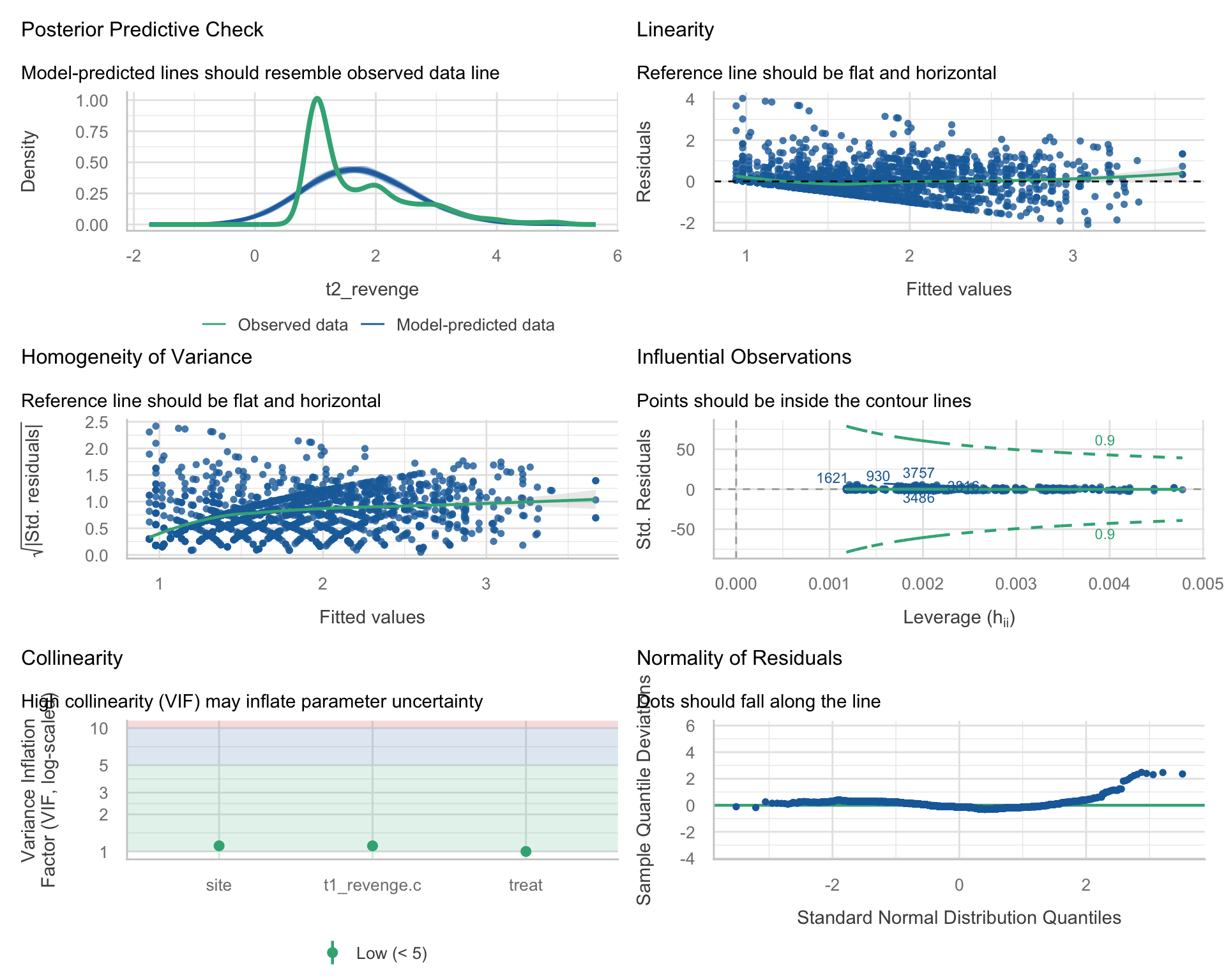
The new panel is the top left. Each blue curve is a dataset simulated from the fitted model: every participant’s prediction plus Normal noise with SD \(\hat{\sigma}\) = 0.69. The green curve is the real follow-up revenge. In the real data, 40% of people sit at exactly 1, the green spike. The simulations can’t produce a spike, and they put about 21% of their scores below 1. ROS (Section 11.4) calls comparing simulated data with the real data “the most fundamental way to check model fit.”
The other five panels repeat Parts 1–3. The one that looks different is normality: it’s a detrended Q–Q plot (the Module explains why), so revenge’s right skew shows as dots rising above a flat line at the upper end.
2 · The result to report. Diagnostics usually earn a few sentences in the Results, after the main result. Following the Module’s template, for revenge:
Regression diagnostics supported the reported treatment estimate. The residuals were right-skewed and their spread increased with the predicted score, consistent with the many responses at the scale’s floor (40% of follow-up scores were 1); given the sample size (N = 3,964), the skew does not threaten coefficient inference. Heteroscedasticity-robust (HC3) standard errors changed the treatment-effect SE by 0.1%, though the baseline-revenge slope’s SE grew by 28%. An exploratory treatment × baseline-revenge interaction indicated a larger reduction at higher baseline revenge (b = −0.26, 95% CI [−0.31, −0.22]; an estimated −0.08 points at the scale’s floor vs. −0.61 at a baseline of 3), consistent with moderation, a floor effect, or both; the additive estimate is therefore an overall summary across baseline levels. No observation approached a Cook’s distance of 1 (largest D = 0.008), and all variance inflation factors were below 1.5.
Notice what it includes: which diagnostics, what they showed, why the departures don’t undermine the estimate, the one substantive finding disclosed, and influence and overlap in one clause.
Wrapping up
What today covered, with revenge
| The Module’s idea | Today’s revenge result |
|---|---|
| Plot the data with the fitted model | At baseline 1 the model’s workbook–waitlist gap is 0.35; the real one is 0.08 |
| The residual–fitted plot: the wedge vs. the smoother | Wedge at the bottom left (the floor); smoother bends gently, 0.19 to −0.15 to 0.10 |
| Additivity | The workbook’s effect: −0.08 at baseline 1 vs. −0.77 at 3.6, recovering both groups’ workbook–waitlist gaps |
| Normality: the Q–Q plot | Skewed right (1.13); matters for one person’s prediction, not the coefficient |
| Equal variance and robust SEs | Spread 0.51 → 0.91; robust ÷ classical SE for the treatment effect: 0.999 |
| Influence and multicollinearity | Largest Cook’s D 0.008; treatment VIF 1.00 |
| check_model()’s predictive check (optional) | Real data: 40% at 1; simulations: 21% below 1 |
| When violations matter | The estimate and its CI survive; its meaning narrows to an overall summary, and individual predictions are unreliable |
What’s next.
Wednesday’s lab finishes the Bread + Peace analysis: you’ll check your final model’s assumptions and see why your final forecast is last week’s.
After Thanksgiving week, Exam 3 covers Part 3: the written part on Mon Nov 30 and the WebR coding part on Wed Dec 2.