install.packages(c(
  # Core — the language toolkit, and project-relative file paths
  "tidyverse", "here",

  # Rendering — what turns a .qmd into an HTML report. RStudio usually offers
  # to install this the first time you render; listing it here means you have
  # it either way.
  "rmarkdown",

  # Importing data that isn't already in R's own format
  "haven", "readxl", "labelled",

  # Describing data and building tables
  "skimr", "gtsummary", "gt", "flextable", "scales", "DT",

  # Visualization helpers that sit on top of ggplot2
  "patchwork", "ggrepel", "ggtext", "GGally", "corrplot", "corrr",
  "gridExtra", "highcharter", "gganimate",

  # Inference and effect sizes
  "infer", "broom", "effectsize",

  # Regression, model diagnostics, and marginal effects
  "marginaleffects", "performance", "car", "sandwich", "estimatr",

  # Complex survey data (NHANES, NSDUH)
  "survey"
))Introduction to the Tools
Learning Objectives
By the end of this Module, you’ll have the full tool stack set up and know how the pieces fit together — the foundation every lab and project for the rest of the semester builds on. Here’s what you’ll be able to do:
- Set up R and RStudio on your own machine, verify that RStudio’s bundled Quarto is ready, and confirm each piece is working
- Open the PSY 652 course project in RStudio and find your way around the four-pane layout (Source, Console, Environment, Files / Plots / Help)
- Recognize the elements of a Quarto notebook — the YAML header, section headings, prose, and code chunks — and render a
.qmdfile to HTML - Understand the difference between an R function and an R package, and use library() to load a package into a session
- Use here::here() to write portable, project-relative file paths that work on any machine
- Follow a small set of clean-code conventions (pipe-first, named arguments) that keep your notebooks readable
- Set up GitHub Desktop and connect it to your GitHub account
- Work through the four version-control moves — pull, edit, commit, push — and use them to back up your work
- Know what doesn’t belong in a Git repository (data files,
.Rproj.user/,.Rhistory) - Use Posit Cloud as a fallback if local install doesn’t cooperate
Overview
Most of what you’ll do in PSY 652 happens through four tools:
- R — the language you’ll write analyses in. R is free, open-source, and one of the standard tools for statistical research in the social and behavioral sciences.
- RStudio — the workshop you’ll do that writing in. RStudio is an integrated development environment (IDE) — the code editor, the running R session, and a window onto your files and plots, all in one place. Like R, it’s free.
- Quarto — the document system that lets a single
.qmdfile mix prose, code, and the code’s output. Every Module page, lab handout, and lecture activity on this website is a rendered Quarto document. You’ll write your lab notebooks and your group-project deliverables the same way. - Git + GitHub — the version-control layer. Git is software that records the changes you choose to commit; GitHub is a website that stores the commits you push, giving you a cloud copy and a way to share work with others. We’ll use GitHub Desktop as the gentle on-ramp.
The course tool stack at a glance
| Tool | Role | You’ll install | You’ll use it for |
|---|---|---|---|
| R | Statistical computing language | Yes — on your machine | Every analysis, every chart, every test |
| RStudio | The IDE — your “workshop” | Yes — on your machine | Writing R code and Quarto documents |
| Quarto | The document system | No — comes bundled with RStudio. You’ll just verify it’s ready. | Every lab notebook, every project deliverable |
| GitHub Desktop | Version control UI | Yes — on your machine | Backing up your work, sharing with collaborators |
| Posit Cloud | Browser-based RStudio (fallback) | No install needed | Backup if local install stalls |
You’ll install R, RStudio, and GitHub Desktop locally on your own laptop — three downloads. In most current RStudio installations, Quarto is already available through RStudio, so once RStudio is in place you usually just need to verify that Quarto responds when called. We’ll keep Posit Cloud in our back pocket as a fallback if any local install fails (see the backup-path section toward the end of this Module) — but the default plan is everything-on-your-machine. Local installs give you the same workflow you’ll use after the course ends, and let you do most of your analysis and writing offline once R, RStudio, the packages, and the course files are in place. (Pushing to GitHub and installing new packages still need a connection.)
What you need to know today
You do not need to understand every detail on the first read. Your job today is to internalize the map: R is the language, RStudio is where you work, Quarto is where you write analyses, and GitHub backs up your work. The details — what an argument is, what a pipe does, what .gitignore is for — will become familiar as we use them throughout the semester. If a section feels dense, that does not mean you’re behind; it usually means you’re meeting an idea for the first time. Finish the section, take a breath, and move on. The Wednesday lab is where a lot of this stops feeling abstract and starts feeling usable.
Your setup checklist for today
By the end of this page, you should have:
You do not need to make your first commit alone — we’ll do that together in the Wednesday lab.
Install R
R is the language. You install it once, and after that you interact with it through RStudio rather than directly: opening RStudio starts and manages an R session for you.
The installers in the steps below will walk you through a series of screens with options. Every time we say “accept the defaults,” we mean: click Next or Continue on every screen without changing anything. For this course, use the default installation settings unless these instructions or the lab instructor tell you otherwise. If the installer presents an option we haven’t anticipated, keep the default — or take a screenshot and ask in lab.
- In your browser, go to cran.r-project.org.
- Click “Download R for Windows”.
- Click “base” (the link near the top — it’s the standard install).
- Click “Download R-X.Y.Z for Windows” (the big link at the top of the page; X.Y.Z is the current version number).
- Run the downloaded
.exefile. Accept the defaults for every screen of the installer. - When the installer finishes, R is installed. You won’t open R directly — RStudio will find it for you.
- In your browser, go to cran.r-project.org.
- Click “Download R for macOS”.
- Choose the right installer for your Mac. If you’re on Apple Silicon (M1, M2, M3, M4, or later), pick the
.pkgwhose filename includesarm64. If you’re on Intel (older Macs), pick the.pkgwhose filename includesx86_64. Unsure? Click the Apple menu → About This Mac and look at the “Chip” line — if it lists an M-series chip, you wantarm64; otherwise you wantx86_64. - Run the downloaded
.pkg. Accept the defaults. - When the installer finishes, R is installed. You won’t open R directly — RStudio will find it for you.
Install RStudio
RStudio is the workshop. This is the application you’ll actually open every time you sit down to work.
WarningIf your operating system is older than the installer wants
Current RStudio Desktop releases require a fairly recent version of Windows or macOS, and the exact cutoff shifts over time as Posit updates its builds. If the current installer tells you your computer is too old, do not panic. Two paths forward:
- Use Posit Cloud for the first lab (see the backup-path section toward the end of this Module). You’ll be up and running in five minutes.
- Email the lab instructor — we can either find an older compatible RStudio release for your machine or keep you on the cloud backup for the semester. Either way, you won’t be left out.
- In your browser, go to the RStudio IDE downloads page. The link jumps you directly to the Install Links section of Posit’s docs.
- Under the Direct Downloads (Open Source) subsection, find the row labeled Windows. The download link is a filename that looks like
RStudio-X.Y.Z-NNN.exe(whereX.Y.Zis the current version number). Click it to start the download. - Run the downloaded
.exe. Accept the defaults. - When the installer finishes, launch RStudio from the Start menu.
- The first time RStudio opens, it should auto-detect the R installation from the previous step.
- In your browser, go to the RStudio IDE downloads page. The link jumps you directly to the Install Links section of Posit’s docs.
- Under the Direct Downloads (Open Source) subsection, find the row for the macOS download (its label shows the minimum macOS version Posit currently supports). The download link is a filename that looks like
RStudio-X.Y.Z-NNN.dmg(whereX.Y.Zis the current version number). Click it to start the download. - Open the downloaded
.dmgfile. Drag the RStudio icon into your Applications folder. - Open Applications and launch RStudio. (The first time you launch, macOS may ask you to confirm you really want to open an app downloaded from the internet — click Open.)
- The first time RStudio opens, it should auto-detect the R installation from the previous step.
Quick check · Did R install correctly?
Open RStudio. Find the Console pane — it’s the pane on the left, on the first tab, labeled Console. (You may see it described elsewhere as the bottom-left pane. That’s where it sits once you have a document open; right now, with nothing open, the Console fills the whole left side of the window.) Click into it and type:
R.version.string…and press Enter. You should see something like "R version 4.X.Y". If you see that, R and RStudio are talking to each other. If you see an error, contact the lab instructor.
Verify Quarto is ready
Good news — you usually don’t need to install Quarto separately. Recent versions of RStudio include a bundled copy of Quarto for rendering .qmd files, which is all you’ll need for this course. The practical question is simply: can your setup render a Quarto document? The most direct way to find out is to render one.
The check that matters · render a sample document
You don’t need to understand Quarto yet — you’ll create a tiny throwaway document and ask RStudio to render it. If RStudio produces an HTML preview, your setup is ready.
- In RStudio’s top menu, click File → New File → Quarto Document…
- A small dialog appears asking for a title and output format. Don’t change anything — just click Create.
- An untitled document opens in the Source pane with some sample content (a title, a couple of headings, a small code chunk). You don’t need to understand any of it yet.
- Look for a yellow bar across the top of the document reading “Package rmarkdown required but is not installed.” On a fresh machine you will almost certainly see it, either now or the moment you click Render. Click Install on the right-hand side of that bar and wait — the installation runs in the Console and takes roughly 30 seconds. Let it finish before going on. Rendering will fail if you skip this, and the error it produces looks alarming but only means this step was missed.
- Find the Render button near the top of the Source pane — it shows a right-pointing arrow icon next to the word Render. Click it.
- RStudio will prompt you to save the file before rendering. Save it anywhere convenient (your Desktop is fine) with any filename ending in
.qmd—test.qmdworks. - Quarto will run for a few seconds, then a rendered HTML preview should open in a new window or in RStudio’s Viewer pane.
If the preview opens, Quarto is working for this course. Close and delete test.qmd afterward — it was only a check.
If the render fails, read the error message and copy it somewhere you can paste it later, then bring it to lab. A render can fail for several reasons that have nothing to do with Quarto being missing — an R package that didn’t install, a file-permission problem, malformed YAML — and installing another copy of Quarto will not fix any of those. Install the standalone CLI (below) only if the error specifically says Quarto itself cannot be found.
Optional · install the standalone Quarto CLI
You do not need this for PSY 652 — the bundled Quarto inside RStudio handles every notebook and project deliverable. The standalone CLI is worth installing only if you want:
- A newer standalone Quarto release, when one is available
- The ability to run
quarto renderoutside RStudio (in a Terminal, or with the VS Code Quarto extension if you ever switch editors) - An independent update path — you can update Quarto without updating RStudio
If any of those describes you, the install is straightforward. Each version below ends by checking the result in RStudio’s Terminal — the tab sitting next to the Console. The Console takes R commands; the Terminal takes system commands, and quarto --version is one of the few things in this course that belongs there.
- In your browser, go to quarto.org/docs/get-started.
- Click “Download Quarto CLI” for Windows.
- Run the downloaded
.msi. Accept the defaults. - In RStudio, click the Terminal tab, type
quarto --version, and press Enter. It should report the standalone version you just installed. (If it still sayscommand not found, the Terminal is running a shell that started before the install and has not picked up the newPATH. Close that Terminal tab and open a new one with Tools → Terminal → New Terminal, or restart RStudio, then try again.)
- In your browser, go to quarto.org/docs/get-started.
- Click “Download Quarto CLI” for macOS.
- Open the downloaded
.pkg. Accept the defaults. - In RStudio, click the Terminal tab, type
quarto --version, and press Enter. It should report the standalone version you just installed. (If it still sayscommand not found, the Terminal is running a shell that started before the install and has not picked up the newPATH. Close that Terminal tab and open a new one with Tools → Terminal → New Terminal, or restart RStudio, then try again.)
Set up your course project
The course materials live in a downloadable bundle called PSY652_project.zip. It contains:
- a
PSY652_project.Rprojfile — the project anchor that RStudio recognizes - a
data/folder pre-populated with the datasets you’ll use across the semester - a
documentation/folder — right now it holds only a bibliography file. You will fill it yourself over the semester with data provenance notes and your own codebooks, starting with the group projects - a
programs/folder where you’ll write your lab notebooks and project deliverables. Inside you’ll find a pre-built.qmdfor each of the first four weekly labs (m02_lab.qmdthroughm05_lab.qmd) andm08_paper.qmd— a manuscript skeleton for Module 8, which ships prebuilt because it uses an APA formatting extension that has to travel with it. (The two group projects live in their own separate repositories, each with its own starter download, so their skeletons are not here.) There is alsolab_template.qmd, a clean skeleton for building a notebook from scratch, andlab_template_annotated.qmd, the same skeleton with every line explained. From Module 6 on, most labs have you build the notebook yourself — starting from the template or from an empty file, as each lab directs. - an
output/folder — a drop point for finalized work you want kept apart from your working files, such as a Project 1 PDF or a Project 2 report. Day-to-day lab renders land next to their.qmdsource inprograms/, not here. Note thatoutput/is deliberately excluded from Git (see the version-control section below), so treat it as local scratch space, not as a submission channel. - a
README.md— a short orientation file describing the folder layout and how to get started (the M02 lab relies on it), plus a.gitignorethat keeps your data and rendered HTML out of Git automatically (we’ll open it in the version-control section below).
Download the course project
The latest project bundle lives at downloads/PSY652_project.zip. Click the link to download, then:
- Find the downloaded file — usually in your
Downloads/folder. The file isPSY652_project.zip. - Unzip it. On Windows, right-click → Extract All. On macOS, double-click. You’ll get a folder called
PSY652_project/. - Move the folder somewhere stable. Recommended: your
Documents/folder. Avoid your Desktop (which can get reshuffled) and avoid syncing it through iCloud / OneDrive (which can cause file-lock weirdness when RStudio is writing). - Open the project in RStudio. Inside the
PSY652_project/folder, double-clickPSY652_project.Rproj. RStudio will open with the project loaded.
When you open a project this way, RStudio sets the working directory to the project folder. The working directory is just R’s answer to a basic question: “if I want to read a file, where am I looking?” By default it’s the folder R was started from. When you open RStudio through a .Rproj file, R is told: “your home base is this project folder.” From then on, any code that reads or writes files using project-relative paths (e.g., here::here("data", "nhanes.Rds")) is starting from the project folder and walking inward — exactly what you want.
This is the heart of reproducibility. Reproducibility in research means: when someone else (or future-you) downloads your code and your data, runs your notebook, and gets the same results you got — no manual tweaks needed. Reproducible analyses don’t rely on hard-coded file paths from one specific laptop, on packages someone happened to have loaded, or on a particular state of the R session that’s now lost. The setup you’ve just done — a portable project folder, an .Rproj file that sets the working directory, and the here() function you’ll meet in a moment — is the foundation that removes several of the most common barriers to reproducibility.
Common setup mistake
The single most common reason a file “won’t load” in Week 1 is opening a lab .qmd by double-clicking it from Downloads/ rather than through the project. Open PSY652_project.Rproj first, then open the .qmd from inside RStudio’s Files pane. That’s what points the working directory at your project folder — so here() paths find your data.
The RStudio four-pane layout
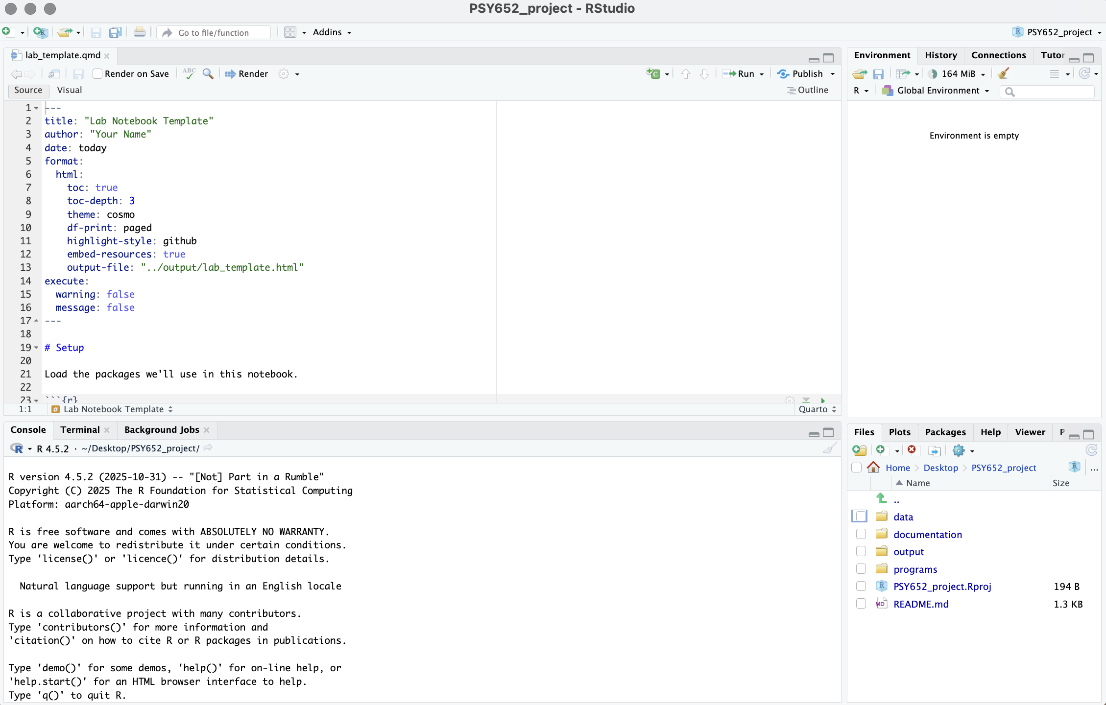
RStudio organizes its window into four panes. Open a file first, or you will only see three — the Source pane appears when there is something to edit. If you have the course project open, click any .qmd file in the Files pane (bottom-right) to bring Source into view; if not, File → New File → R Script works just as well and you can close it afterward. Most conveniently, open m02_lab.qmd in the programs/ folder — you’ll be working in it for the Wednesday lab.
With a file open, you’ll see:
- Source (top-left) — your code editor. You’ll open
.qmdand.Rfiles here. Type code, edit prose, and render documents. Close every file and this pane collapses, handing the whole left side to the Console. - Console (bottom-left) — the live R session. Type one-off R commands here for quick experiments. When you run code from a notebook, R executes it in this session — and, depending on how you run it, the results may appear inline below the chunk, here in the Console, or in the Plots/Viewer pane.
- Environment (top-right) — a list of the objects currently in your R session (data frames, vectors, fitted models). For many objects, you can click their names to inspect them more closely.
- Files / Plots / Help / Packages (bottom-right) — a multi-tab pane. The Files tab is a mini file browser; Plots shows recent charts; Help shows function documentation; Packages lists installed packages.
Install the course packages
R’s power comes from thousands of community-built packages. Think of a package as an add-on that bundles related functions together — one package for plotting, another for tidying data, another for fitting models. Each one adds specialized capabilities on top of base R, the set of functions that ships with R itself.
Before you can use a package, two things have to happen:
- Install it — a one-time download from the internet onto your laptop. Think of this like buying a book and putting it on your shelf.
- Load it — every R session in which you actually want to use the package’s functions. Loading is like taking the book off the shelf and opening it to the page you need.
You install once; you load every session. We’ll do the install now and the loading later, when you’re working in a specific notebook.
This installs every package the course’s modules, labs, and projects use, so you only have to do it once. You will not need all of them in Week 1 — several belong to the regression work in the back half of the semester — but installing the full set now means a lab never stalls on a missing package. They are grouped by what they do, purely so the list is readable; the grouping has no effect on the install. Open RStudio (with the course project loaded), and in the Console, paste this:
The first time, expect this to take a while — often ten minutes or more, since R downloads each package plus everything it depends on. Let it run. You generally only need to do this once on a given computer, and later in the semester you’d re-run it only to pick up an update. Don’t worry about the long stream of messages. When it finishes, scan the output for a line beginning with ERROR: or a note that a package had a non-zero exit status — if the > prompt returns and nothing reports a failed install, you’re done. Bring any installation error to lab. If R asks whether to install a package from source, choose No (the pre-built binary) — source installs can require extra developer tools we don’t need for this course.
Set up global options
Out of the box, RStudio tries to be helpful in a way that quietly undermines reproducible science. When you quit RStudio, it offers to save your workspace — a snapshot of every object currently in your Environment pane (your data frames, your fitted models, your variables) — to a hidden file called .RData in your project folder. The next time you open RStudio, it offers to restore that snapshot, repopulating the Environment pane with all those objects. The pitch is “pick up where you left off.”
In practice, this creates a real problem. Imagine you spend an afternoon wrangling NHANES into a tidy data frame called nhanes — filtering, recoding, dropping columns. You quit. RStudio saves the workspace. Three weeks later you reopen the project and nhanes is right there in the Environment pane. But you have no idea which code produced that version of nhanes. Did you filter to adults only? Was age coded in years or in five-year buckets? Did you drop missing values, or impute them? You can’t tell, because the object came back as a snapshot of memory, not as the output of a script you can re-run. Your code and your Environment have silently drifted apart, and the analysis you submit weeks later may depend on a step you can no longer reconstruct.
The fix is to tell RStudio: never save the workspace on exit, and never restore it on startup. Every R session starts blank. Anything you want available in the Environment has to be produced by code you actually run — code that lives in a .qmd or .R file, that you (or anyone else) can re-run from scratch. Your script becomes the source of truth; the Environment pane is just where the script’s results currently happen to live.
If this feels slightly inconvenient at first, that reaction is normal. Beginners often feel reassured when old objects are still sitting in the Environment pane. But in the long run, a clean start is much safer: it forces your code to be honest about what it needs in order to work.
This is the professional default for reproducible research. The small cost (you re-run your setup chunk at the start of each session) buys you a much better chance that every analysis rebuilds from a clean slate.
To turn it on:
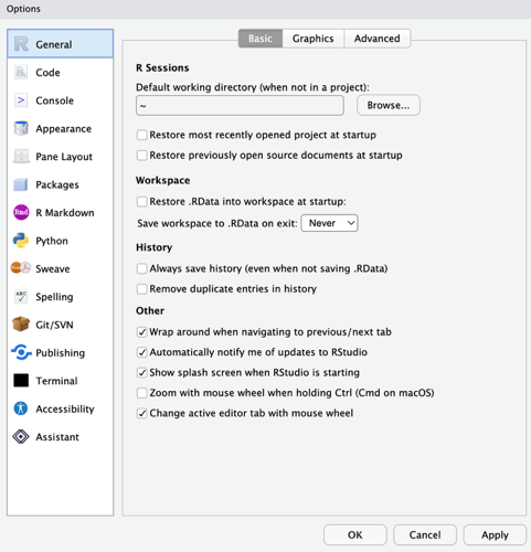
- Select Tools → Global Options
- Click General on the left menu and click the Basic tab
- Under Workspace, uncheck “Restore .RData into workspace at startup”
- Under Workspace, set Save workspace to .RData on exit to Never
- Under R Sessions, uncheck “Restore most recently opened project at startup”
- Click Apply, then OK
Step 5 is the same idea applied to projects rather than objects. Left on, RStudio reopens whatever you had going last time — which sounds convenient until you are working on two courses at once, or you sit down at a lab machine that opens someone else’s project. Off, RStudio starts neutral and you choose the project deliberately, which is also how you avoid saving work into the wrong folder.
What about the other checkboxes on this tab? Leave them alone. The settings above have a real consequence — they’re what keeps your Environment honest about what your code actually produces. The rest (history behavior, tab-navigation wrap-around, update notifications, crash reporting) are preference and telemetry; none of them affects whether your analysis reproduces. The exact list varies between RStudio releases, so if your dialog doesn’t match a screenshot exactly, that’s expected — change only the settings named above.
Your global options dialog box should now look like this:
Done. From now on, every R session starts clean — your scripts and your Environment will stay in sync. (If you already see a file named .RData in your project folder from before you changed this setting, delete it — from now on your code, not a saved snapshot, should recreate every object.)
Your first Quarto notebook
Every analysis you write in this course will be a Quarto notebook — a single .qmd file containing your prose, your R code, and the output of that code (numbers, tables, charts) all woven together. When you render a notebook, you get a clean HTML document that someone can read without needing R installed — the course template bundles its images and styling into that one file, so it’s easy to email or post.
Now let’s look at what one of these notebooks actually looks like in practice. Open the file at programs/lab_template.qmd in your RStudio Source pane. To do that:
- Look at the Files tab in the bottom-right pane of RStudio. You should see the contents of your
PSY652_project/folder listed — including the foldersdata/,documentation/,output/, andprograms/. - Click on the
programsfolder name to navigate into it. - Click on the file
lab_template.qmd. RStudio opens it in the Source pane (top-left), where we’ll do the rest of this walkthrough.
We’ll walk through every element of the file.
The YAML header
The very top of the file looks like this:
---
title: "Lab Notebook Template"
author: "Your Name"
date: today
format:
  html:
    toc: true
    toc-depth: 3
    theme: cosmo
    df-print: paged
    highlight-style: github
    embed-resources: true
execute:
  warning: false
  message: false
---
The triple dashes (---) on the first and last lines tell Quarto: this block is configuration, not content. Each line inside controls one thing about the document:
title,author,date— the text that appears at the top of the rendered page.date: todayfills in the current date automatically every time you render, so you never update it by hand.format: html— render this document to HTML (a web page). The indented lines beneath it fine-tune that HTML:toc: true— build a table of contents from your headings and show it alongside the document.toc-depth: 3— include headings down to level 3 (###) in that table of contents, and no deeper.theme: cosmo— apply a clean, built-in visual theme (its fonts, colors, and spacing). Cosmo is a sensible default; Quarto ships many others.df-print: paged— print data frames as tidy, interactive paged tables instead of as raw console text.highlight-style: github— color-code your R code using GitHub’s familiar syntax-highlighting palette.embed-resources: true— bundle everything the page needs (styles, fonts, images) into the single.htmlfile, so the result is one self-contained file you can email or submit — with no accompanying folder to keep track of.
execute:— options applied to every code chunk in the document; we’ll unpack whatwarning: falseandmessage: falsedo when we reach code chunks below.
By default, Quarto renders a file called foo.qmd1 to foo.html right next to the source — so the rendered HTML for this template lands at programs/lab_template.html. Most Quarto documents open with a YAML block like this one, and every notebook you write in this course will.
Section headings
Below the YAML, sections of your notebook are organized by headings. (The YAML block at the top is a header; the # lines that structure your prose are headings.) Headings come in levels — a single # at the start of a line is a top-level heading (an H1); ## is an H2, one level down; ### is an H3; and so on. Think of them as an outline: an H1 is a top-level section, an H2 is a section nested within it, and an H3 is nested one level further.
# Setup

# Import Data

# Glimpse
These headings populate the table of contents that appears in the right margin of the rendered document. Use them generously — they let your reader (and future-you) navigate quickly. You can view the outline in RStudio too: click the Outline button in the top-right of the Source pane.
Prose
Anything that isn’t inside a code chunk or a YAML block is treated as prose. You write it in Markdown — a simple system for marking up plain text so it renders with formatting. Instead of clicking a “bold” button like in Microsoft Word, you wrap text in special characters, and Markdown turns those characters into formatting when the document renders. The most common patterns:
- Surround text with two asterisks
**on each side to make it bold: writing**important**renders as important. - Surround text with one asterisk
*on each side to make it italic: writing*emphasis*renders as emphasis. - Write
[link text](url)to make a clickable link: writing[Google](https://google.com)renders as Google.
You’ll pick up the rest of Markdown’s syntax as you go — it’s mostly small patterns like this. The full reference is at quarto.org/docs/authoring/markdown-basics.
This is where you explain what you’re doing and why — your interpretations, your reasoning, the substantive story behind the numbers. A good Quarto notebook reads like a research report with the code on display rather than a script with comments stapled on.
Code chunks
The gray boxes are code chunks — the place where your R code lives. A chunk starts with three backticks plus {r} in curly braces and ends with three backticks. A backtick is the small slanted mark ` — on most US keyboards, it shares a key with the tilde ~, just to the left of the 1 key, near the top-left corner. (It’s not a single quote ', which sits next to the Enter key — that’s a different character.) The three-backtick fences tell Quarto: “everything between these two fences is code, not prose.” If this notation looks strange at first, that’s normal; it becomes familiar very quickly once you’ve used it a few times.

You don’t have to type those fences by hand. RStudio can insert them for you: click the green +C button in the toolbar at the top of the Source pane and choose R, or press Cmd+Option+I (Mac) / Ctrl+Alt+I (Windows). Either way an empty chunk appears at your cursor with both fences already correct, waiting for code. You’ll do this for the first time in this week’s lab, and it becomes routine from M06 on, when you start building each week’s notebook from lab_template.qmd.
Chunk options · controlling what each chunk does
Every code chunk can carry a few options that tell Quarto how to handle it — whether to show the code or just its result, what size to draw a figure, whether to print R’s warnings alongside the output. Options sit at the very top of the chunk, each on its own line prefixed with #| (a hash mark followed by a pipe).
A chunk with options looks like this:
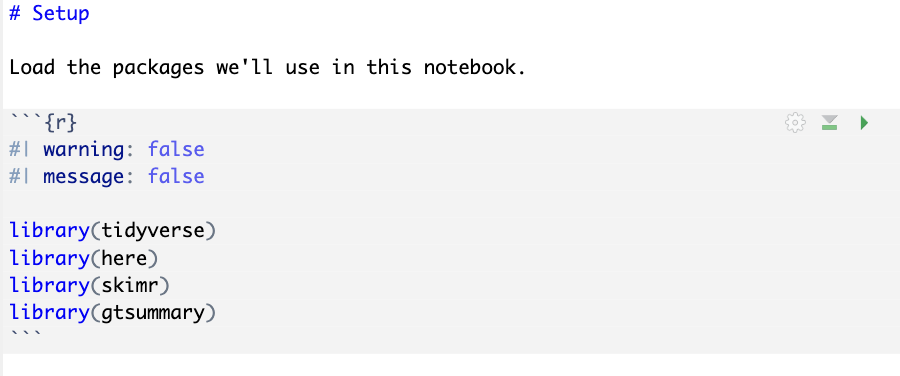
The two options you’ll meet most often control what R’s chatter does to your report:
message: falsehides R’s informational messages — the “Attaching core tidyverse packages…” block tidyverse prints on load, for instance. Most of these are startup noise your reader does not need. A few carry information worth knowing, though, so “informational” is not a synonym for “ignorable” — see the box below.warning: falsehides R’s warnings — R flagging something that might be a problem, like a chart that quietly dropped rows with missing values. Unlike messages, a warning can carry real information, so treat it with more care (see the box below).
Set them once, globally
Rather than repeat #| lines on every chunk, you can set options once for the whole document in the YAML header’s execute: block — the two lines you saw in the YAML earlier:
execute:
  warning: false
  message: false
Every chunk then inherits them automatically, which is how the lab template is set up — you set the usual reporting defaults once, then override them when you need to inspect something. If you want one chunk to behave differently, put a #| option on that chunk and it overrides the global default. For example, #| warning: true un-hides warnings for a single chunk while you debug it.
Reading warnings and messages while you work
These settings suppress warnings and messages in the rendered report — and RStudio may honor them when you run a chunk interactively too, so do not assume every warning stays visible while you work. When you are chasing a problem, temporarily override the defaults on that chunk with #| warning: true and #| message: true, or run the line on its own in the Console, where nothing is suppressed.
When you do see R’s chatter, the habit to build is to read it and decide whether it needs action:
| What you see | How to read it | What to do |
|---|---|---|
| “Attaching core tidyverse packages…”, “masked from…” | Routine startup message | Nothing — this is what loading a package looks like. |
“summarise() has grouped output by…” |
Informational, but it can matter | It is telling you the result is still grouped, which changes what a later mutate() or summarize() does. Decide whether you want that; if not, add .groups = "drop" inside summarize() or follow with ungroup(). |
| “Removed 12 rows containing missing values” on a plot | Actionable (warning) | Rows were silently dropped from the chart — check why they’re missing and whether dropping them is fine. |
| “NAs introduced by coercion” | Actionable (warning) | R couldn’t turn something into a number — usually a stray text value or typo in a numeric column. Track it down. |
A warning isn’t a crisis — most are benign once you understand them — but it deserves a ten-second look before you trust the result. And by default an execution error stops the render and Quarto reports where it happened, so code that fails to run cannot slip through unnoticed. What that does not catch is code that runs perfectly and produces the wrong answer — for that, there is no substitute for reading your output and checking it against what you expected.
There are many more chunk options — hiding the code while keeping its output (echo: false), setting a figure’s size (fig-width: 6, fig-height: 4), naming a chunk (label: setup) — and we’ll meet them as the course goes on. The full list lives in the Quarto documentation.
Functions, packages, and the pipe
Before we look at the chunks themselves, we need to define three terms that show up in every line of code you’ll write: function, package, and pipe.
What is a function?
A function is a piece of pre-written code that performs one specific task. You don’t write it from scratch — someone else already did, you just call (i.e., use) it by name. The function itself is the stored set of instructions; the function call is the code you write to run it. A call usually has three visible parts:
- a name — what you type to call the function (e.g.,
mean,read_rds,library) - a pair of parentheses
()immediately after the name — this is what tells R “go ahead and run this function” - zero or more arguments inside the parentheses — the inputs that tell the function exactly what to do
Here’s a concrete example. The function mean() computes the average of a set of numbers. Say you store three blood-pressure readings in an object called SBP and want their average — you call the function and tell it which values to average:
SBP <- c(120, 128, 134) # three example readings, stored in an object called SBP
mean(x = SBP)
That # on the first line starts a comment: R ignores everything after the # on that line, so it’s a handy place to leave a note about what the code does — for a collaborator, or for your future self. The same trick lets you comment out a line by putting a # in front of it, switching it off without deleting it. Comments never change what the code actually runs.
In the second line, mean is the function’s name, the parentheses say “run this function,” and x = SBP shows the input you’re giving it. Here, x is the argument name and SBP is the value you are supplying for that argument. You do not need to memorize argument names for every function right now; the important point is that functions often need inputs, and the code inside the parentheses is where those inputs go.
A common point of confusion · when names can be left off
You’ll often see the same line written two different ways:
mean(x = SBP) # name written explicitly
mean(SBP)     # name omitted — same result here
Both lines do exactly the same thing. R often lets you omit the argument name when the meaning is unambiguous, especially for the first argument. That is why you will regularly see code like mean(SBP), glimpse(nhanes), and library(tidyverse).
In this course, the rule of thumb is simple: when a function has several arguments, naming them usually makes code easier to read. When a function has one obvious input, omitting the name is common and perfectly fine. If this distinction feels subtle on first read, that’s okay — it becomes much clearer once you’ve written and run a few functions yourself.
Functions with no arguments and functions with many
Some functions need no arguments at all — they do one fixed task, and you just call them with empty parentheses. Some take one simple argument like mean() above. Some take many arguments, and you specify each one by name: mean(x = SBP, na.rm = TRUE) says “compute the average of SBP, and also: when you encounter missing values (NA), drop them before averaging.” You’ll meet all three flavors as the course goes on.
What is a package?
R comes with a core collection of built-in functions — the ones available the moment you start R, known collectively as base R. Base R can do a lot, but it does not include every function ever written. For specialized tasks — making a chart, fitting a regression, writing a publication-ready table — the R community has built packages: collections of related functions you can add on top of base R.
Each package bundles functions that do related work. A few examples you’ll meet this semester:
- ggplot2 — functions for making charts
- dplyr — functions for filtering, grouping, and summarizing data
- readr — functions for reading data files (including read_rds())
- here — the function here() for building portable file paths
(The first three are part of a larger family of packages called the tidyverse — installing tidyverse installs its component packages, and loading it attaches the core ones — ggplot2, dplyr, readr and a few more — in a single step. We’ll lean on the tidyverse heavily.)
As covered above, two things have to happen before a package’s functions are usable:
- Install the package (the one-time download from the internet to your laptop), which you already did when you ran install.packages() earlier in this Module.
- Load the package in the current session (the every-session step), which you do with the library() function at the top of your notebook:
library(tidyverse)
library(here)
library(skimr)
Each line above calls the library() function once, passing the name of one package as the argument. After all three lines run, the functions from here and skimr, plus those in the core packages that tidyverse attaches, are available to use in the rest of your notebook. By convention, library() calls live at the very top of a notebook so a reader can tell at a glance which packages the analysis depends on.
You’ll sometimes see a function written with its package name and two colons in front of it — like here::here() instead of plain here(). The package::function() form just means “the here() function, from the here package,” said out loud. Once you’ve loaded here with library(), here::here() and here() are the same function, and you can treat them as interchangeable — that’s why you’ll see both across this course. The :: form has two uses. It lets you borrow a single function without a library() call first. And it settles which package you mean when two loaded packages define a function of the same name: with plain here(), R uses whichever package you loaded last, whereas here::here() always means the one from here. That ambiguity is real in general — the plyr package, for instance, also exports a here() — but it never arises in this course, because we never load a package that collides with the ones we use. You don’t need to write :: yourself in this course — plain function names are our default — but now you’ll recognize it in other people’s code.
The pipe |>
The pipe is a small piece of punctuation — two characters, |> — that lets you chain functions together left-to-right, in the same order you’d describe a recipe out loud. The pipe is technically called an operator (a symbol that performs an action) — but for our purposes the only thing to remember is the rule it follows:
Take whatever sits on the left of the pipe, and feed it as the first argument into the function on the right.
So nhanes |> glimpse() is read as: “take the nhanes data frame, then hand it to the glimpse() function.” When you see |>, say “then” in your head — it almost always parses correctly.
The real payoff is when you chain several steps together. Suppose we want the mean systolic blood pressure for adults, grouped by marital status:
nhanes |>
  filter(age >= 20) |>
  group_by(marital_status) |>
  summarize(mean_SBP = mean(SBP, na.rm = TRUE))
Read this as: “take nhanes, then filter to just the adults (rows where age is 20 or older), then group by marital status, then within each group compute the mean of SBP.” Notice how the thens in the English description line up exactly with the |> symbols in the code. The pipe |> lets you write code in the same order you’d describe what it does.
For contrast, here’s the same operation written without the pipe:
summarize(group_by(filter(nhanes, age >= 20), marital_status),
  mean_SBP = mean(SBP, na.rm = TRUE))
To understand what this code does you have to start at the innermost call, filter(), and read outward — the first operation is buried deepest. Once you stack three or four steps, the code gets hard to follow fast. The pipe is what saves you from that.
We’ll write code with the pipe in this course.
Loading your data · the assignment operator, here(), and read_rds()
The PSY 652 course project that you set up earlier in this Module includes a data/ folder, and inside that folder sits a file called nhanes.Rds — the NHANES dataset we’ll work with for the rest of this Module (and several Modules after). Right now that file is just sitting on your laptop’s hard drive. Before R can do anything with the data — look at it, filter it, plot it — the data has to be loaded into your R session. The two states are different in an important way:
- On disk. The file
data/nhanes.Rdsexists as bytes on your laptop’s storage — but nothing has told R about it yet, and until you import it your code cannot touch its rows or columns. The file is dormant. - In your R session (in memory). Once you load the file, R holds the data as a live object — a data frame your code can filter, summarize, plot, or pass to other functions. This is where every other line of your analysis acts.
The act of moving data from disk into your R session is called importing. Almost every analysis you’ll ever write begins with an import step, because the data has to be live in memory before your code can work with it.
For R’s native single-object file format — files whose names end in .Rds — a common function for importing is read_rds(). Here is the line from the template’s Import Data chunk that imports the NHANES file:
nhanes <- read_rds(here("data", "nhanes.Rds"))If this line looks busy, that’s normal. Early in the semester, many useful R lines will look like several small ideas packed together. The goal isn’t to read it instantly; the goal is to learn how to unpack it one piece at a time.
Three pieces are doing the work together — the assignment operator <-, the here() function, and the read_rds() function. Let’s slow down on each one.
The assignment operator · <-
R’s assignment operator is <- (read aloud: “gets”). It takes whatever sits on the right and gives it a name — the name on the left. So the line above says: “call read_rds() on this file, and store the result under the name nhanes.”
After this line runs, nhanes is a name R recognizes. Anywhere later in your notebook that you write nhanes, R will look up the thing you stored and use it. In this case, the thing stored is a data frame — R’s standard tabular structure, with one row per observation (one NHANES participant) and one column per variable (age, marital status, SBP, etc.).
You can choose any name you like. Writing my_data <- or survey <- instead of nhanes <- would work equally well — though if you change the name on the left, you have to change every later line that refers to it. By convention, course materials use nhanes so that everyone’s code matches.
R is case-sensitive
R treats upper- and lower-case letters as completely different characters. That is true for everything you type — object names, function names, package names, and column names alike:
nhanesandNhanesare two different names. Store your data asnhanesand then ask forNhanes, and R reportsobject 'Nhanes' not found— it has no idea they were meant to be the same.read_rds()works;Read_rds()andREAD_RDS()do not — R sayscould not find function.- A column called
SBPcannot be reached by typingsbp.
Most beginner “why won’t this run?” errors are a single wrong capital letter. So when R can’t find something you’re sure exists, check the case first: match what you type to what you named, letter for letter. (This is also why consistent naming helps — the course mostly sticks to lowercase names like nhanes and life_expectancy so there’s less to remember at the beginning.)
The here() function · finding the file
To load a data file, R needs to know where on the laptop the file lives. The straightforward approach is to write the full path:
nhanes <- read_rds("/Users/your_name/Documents/PSY652_project/data/nhanes.Rds")This works on your laptop. It does not work the moment you share the project with anyone else — your collaborator doesn’t have a your_name folder inside their /Users/, and Windows machines don’t have /Users/ at all. Hard-coded paths break as soon as the project moves.
The here package solves this. The here() function looks up the root of your project — the folder containing your .Rproj file — and builds paths relative to that root. So:
here("data", "nhanes.Rds")means “from the project root, go into the data folder, find the file nhanes.Rds.” That instruction is independent of where the project folder itself sits on a given machine. Anyone who opens your .Rproj and runs your code gets the right path automatically — your laptop, your collaborator’s, your future self after a hard-drive transplant. This is the single biggest reason your code will keep working when the project travels.
Wrapping every file path in here() is the habit that makes your code portable. Hard-coding a path that starts with /Users/... or C:\Users\... works only on your machine — here() makes it work everywhere.
The read_rds() function · reading the file
read_rds() takes a path to an .Rds file and returns the R object stored in that file. The .Rds extension is one of R’s native, compact data formats — fast to load and preserves R’s data types automatically (so a column of factors stays a factor, a column of dates stays dates, etc.). In principle a .Rds file can store any R object (a single number, a fitted model, a list); in this course, each .Rds file stores a data frame. All the PSY 652 datasets are distributed as .Rds files in the data/ folder of the course project.
What you’ll see after running this chunk
When you run the chunk containing this line — by clicking the green arrow, or with Cmd/Ctrl + Shift + Enter2 — two things happen:
- R reads the file at
data/nhanes.Rdsand builds a data frame from it in memory. - R stores that data frame under the name
nhanes, and you’ll seenhanesappear in the Environment pane (top-right). Click on its name and a tab opens showing the rows and columns — that’s your dataset.
From this point on, every line of code later in the notebook that mentions nhanes is referring to that in-memory data frame. The template’s Glimpse chunk, nhanes |> glimpse(), runs the glimpse() function on it — you’ll learn what glimpse() reports in M03 and M04, but for now know that it prints a tidy one-line-per-column overview of what’s in the data frame.
Running code · inline and rendered
A Quarto notebook lets you see your code’s results in two different ways. The everyday one is inline — running chunks one at a time as you develop. The polished one is rendering — letting Quarto run every chunk in order and weave the results into a clean HTML document. You’ll use both, but most of your time is spent running inline.
Inline · the everyday workflow
To run a single chunk, click the green arrow in the chunk’s top-right corner (or put your cursor anywhere inside the chunk and press Cmd/Ctrl + Shift + Enter). The chunk runs in your live R session, and its output — a glimpse, a summary table, a plot — appears right below the chunk in the notebook.
Two things to watch as you do this:
- The Environment pane (top-right) populates as you run chunks. A chunk containing
nhanes <- read_rds(here("data", "nhanes.Rds"))creates an object namednhanes— and you’ll see it appear in the Environment pane the moment the chunk finishes. Anything in that pane is live and available to your next line of code; an object you expected to see and don’t may never have been created in this session, or may have been removed. The Environment pane is how you confirm which named objects currently exist — not everything your code did, since code can also print results, draw a plot, or write a file without creating an object at all. - You can also run individual lines without running the whole chunk. Put your cursor on a line and press
Cmd/Ctrl + Enter. That single line runs in the Console and its result prints there. Useful when you’re trying to debug one statement inside a longer chunk.
This is the loop you’ll live in for most of every work session: write a few lines, run the chunk (or the line), look at the result, iterate. Fast feedback, no waiting for a full document build. (If a keyboard shortcut doesn’t work on your machine, everything here is also available from the green Run button in the chunk’s corner and the Run menu at the top of the Source pane.)
Rendered · the polished artifact
When you’re ready to produce the version someone else will read, click the Render button at the top of the Source pane (look for the right-pointing arrow icon). Quarto then runs the document in a separate, clean R session and writes the rendered HTML as lab_template.html right next to the .qmd file in the programs/ folder. RStudio’s preview pane usually opens the rendered HTML automatically so you can see the result.
This separation matters. Objects that happen to exist in your current interactive session do not automatically carry over into the render. That’s a feature, not a bug: it means rendering checks whether your notebook truly contains all the code it needs to reproduce the analysis from scratch.
The project’s output/ folder is a drop point for work you’ve decided is finished — an exported figure, a table you want to reuse — kept apart from the files you’re still iterating on. Day-to-day lab renders land next to their source for quick iteration.
Both output/ and all *.html files are excluded from Git, and the reason is the same in each case: they are generated from the .qmd files in programs/, so committing them would store a second copy of something Git already lets you rebuild. What GitHub preserves is the source needed to regenerate them. Submit finalized deliverables through Canvas (or wherever the assignment specifies) — not by pushing them to your repository.
This is what you do at the end of a coherent stretch of work, before submitting a lab, before sharing with a collaborator. The render’s “fresh-session, run-everything-in-order” behavior is also a built-in correctness check: if a chunk depends on something you defined and then deleted, the render will catch it where the inline workflow had been silently using the leftover object.
The render-edit-render loop
Real analysis happens in this loop: edit your .qmd → run inline as you develop → render periodically → look at the rendered output → edit again. Inline runs are your minute-to-minute feedback; rendering is the periodic “does the whole thing still build from scratch?” check. The rendered HTML is the artifact someone else reads; the .qmd is what you maintain.
When the session feels stale · Restart R and clear outputs
R remembers everything you’ve done in a session — every loaded package, every variable you assigned, every dataset you read in. Most of the time this is helpful. Occasionally it’s the source of a bug: a function you wrote and edited still has the old version in memory; a data frame still holds yesterday’s filtered rows; a package loaded earlier is masking a function name you now want from a different package. The fix is a fresh session.
Needing to restart R is not a sign that you’ve broken something unusually badly. It is a normal part of working in R, and experienced users do it all the time.
- Session → Restart R (or
Cmd/Ctrl + Shift + F10) clears your Environment, unloads all packages, and gives you the same blank slate that a render starts from. Re-run your chunks from the top and the bug usually surfaces. - The little broom icon in the Console pane clears the printed Console history without restarting R. This is the safe one to reach for when the Console has scrolled past usefulness but you do not want to lose your loaded data.
- Be careful with the broom icon in the Environment pane. That broom does not just clear printed output — it removes the objects R is currently holding in memory (your loaded data frames, your fitted models, etc.). Your saved files on disk are untouched, but every object in the live R session is wiped, and you’ll have to re-run your chunks to recreate them. Use it deliberately, not accidentally.
A good habit: before you click Render, restart R and re-run your chunks inline. If everything still works from scratch, the render will too.
Backup path · Posit Cloud
If you can’t get the local install working — most often because of a corporate-managed laptop that won’t let you install software, or a Chromebook that doesn’t run RStudio Desktop — Posit Cloud is the fallback. The short version is below; the full walkthrough, including the one step people skip, is on the Posit Cloud page.
WarningUsing Posit Cloud as a backup
Posit Cloud is RStudio running in your browser. The interface is nearly identical to the desktop version; the main differences are that files live on Posit’s servers (not on your laptop) and the free tier includes a limited number of compute hours per month — enough for most students.
Setup:
- Visit posit.cloud and click Sign up to create a free account.
- Open the PSY 652 cloud project. The link opens a temporary copy.
- Click “Save a Permanent Copy” at the top of the window. From now on, you’ll work in your own copy.
- The cloud project is pre-populated with the course datasets and the same lab template you’d get from the local zip — so the lab walkthroughs in subsequent Modules work identically.
What to know:
- The free tier’s monthly compute hours may be adequate to complete your work. If you need more, Posit offers paid plans with additional hours for a small fee — check Posit Cloud’s current pricing before upgrading.
Version control with Git + GitHub
Version control does two related things for you. Git records the changes you deliberately commit, which lets you answer questions like what did this analysis look like last Tuesday? Why did I change this line? Can I recover the version of the table that had the right p-value? GitHub stores the commits you deliberately push, so that history lives in two places at once — your laptop and a server somewhere else — and a lost laptop, a dead hard drive, or a spilled coffee doesn’t end your semester.
Read those verbs carefully, because they are the whole story: commit and push are things you do, not things that happen automatically. What you get back is a recoverable history of your tracked project files. Work you haven’t committed, commits you haven’t pushed, and files excluded by .gitignore live only on your computer.
Git is the tool that does the change-tracking. Every time you tell Git “these changes belong together” — by writing a short description and clicking a button — Git records a labeled checkpoint of the tracked files you included in that commit. From then on you can scroll back through the list of checkpoints, see exactly what changed at each one, and return to any earlier version of any file. (That last part is the one people are most surprised by, and it has its own short guide: Going back to an earlier version. You will not need it this week — bookmark it for the afternoon you do.) The collection of checkpoints, together with the files they describe, is called a repository (or repo for short) — essentially, a project folder that Git is paying attention to.
GitHub is the cloud half. It’s a website that stores the commits you have pushed — their full history, and the tracked files they contain — on its servers. Every time you push, the cloud copy catches up to the commits on your laptop. If anything happens to your machine, you can install GitHub Desktop on a new computer, click Clone, and recover the tracked files and commit history you had pushed. The cloud copy is not just a snapshot of the current state; it’s the whole timeline of what you pushed.
One consequence is worth stating plainly, because this course’s setup makes it concrete: anything .gitignore excludes is not on GitHub — and that deliberately includes the course data/ folder. If you restore your project onto a new machine, you get your notebooks and their history back, and you re-download the data separately. Together, Git and GitHub are the standard for managing code-based research.
We’ll use GitHub Desktop — a free, friendly graphical app that puts the four basic Git moves under obvious buttons. If you ever want to graduate to the command line, the underlying Git is the same — but for PSY 652, GitHub Desktop is more than enough.
Before the installation steps, it helps to see why this tool is worth learning at all:
Why every research project should be version-controlled
- Recovery. “Last week’s version” is one click away. No more
analysis_final_v3_REALLY_final.qmd. - Backup. Your project lives in two places — your laptop and GitHub — so a hard-drive failure doesn’t end your semester.
- Audit trail. Every commit has a message and a date. Six months from now, you can read the history and remember why you made each change.
- Collaboration. Your group-project partners can see your changes; you can see theirs. When two sets of changes can’t be reconciled automatically — most often because two people edited the same lines — Git reports a merge conflict and asks you which content should stay, instead of letting one person’s work silently overwrite the other’s.
- Portfolio. If you choose to make some of your repositories public later, GitHub can become a portfolio of your analytic work — searchable, shareable, and a reasonable thing to point at on a CV. Nothing requires you to make work public; many researchers keep their repos private until a paper is submitted.
Install GitHub Desktop
- In your browser, go to desktop.github.com. The page redirects to the official GitHub Desktop landing page.
- Click “Download for Windows (64bit)”.
- Run the downloaded installer. (GitHub Desktop includes the Git tools it needs for the workflow we’ll use in this course, so you don’t need to install Git separately. If you later want to use RStudio’s built-in Git pane or the command line, you may need to install system Git and point RStudio at it.)
- Launch GitHub Desktop.
- In your browser, go to desktop.github.com. The page redirects to the official GitHub Desktop landing page.
- Choose the right download for your Mac. If you’re on Apple Silicon (M1, M2, M3, M4, or later), click “Download for Apple silicon”. If you’re on Intel (older Macs), click “Download for Intel chip”. Unsure? Click the Apple menu → About This Mac and look at the “Chip” line. (If the page no longer asks you to choose Apple Silicon versus Intel, just use the default macOS download GitHub recommends.)
- Open the downloaded file. Depending on your macOS version, GitHub Desktop may launch straight away rather than showing the familiar “drag to Applications” window — both are normal. If it launches without asking, that is fine; carry on.
- Say yes if macOS offers to move the app to your Applications folder. That prompt can appear right away, or not until after you sign in. Whenever it appears, accept it — the app may restart, which is expected.
Create a GitHub account
If you don’t already have one, go to github.com and sign up. Use an email address you’ll keep — your CSU address can work, but a personal address is fine too if you want continuity after graduation.
The quickest route is through GitHub Desktop itself. When it first opens it shows a welcome screen with two buttons: Sign in to GitHub.com if you already have an account, and Create your free account if you don’t — that second button just opens github.com in your browser, so you can do it either way.
Whichever route you take, verify your email when GitHub sends the confirmation link; the account is not fully usable until you do. Then return to GitHub Desktop, click Sign in to GitHub.com, and enter the username and password you just created.
Expect the exact sequence to vary. Depending on your operating system and version, the app may ask to move itself to Applications before you sign in, after you sign in, or not at all; it may restart once; and it may offer to create or clone a repository at the end. None of that is a problem, and you do not need to match a screenshot. What matters is the end state, which the check below describes.
One thing to hold off on: GitHub Desktop will invite you to create a repository, clone one, or open an existing folder — skip that for now. We add the PSY652_project repository together in the Module 2 lab, where any snags get sorted in the room rather than alone at your desk. Quit GitHub Desktop once the check below passes and come to lab.
If you’d rather connect through the menus (or need to re-check later):
- Verify your email (GitHub will send a confirmation link).
- Connect GitHub Desktop to your account. Open GitHub Desktop → File → Options → Accounts (Windows) or GitHub Desktop → Settings → Accounts (macOS) → click Sign in to GitHub.com and follow the browser flow.
Quick check · Is GitHub Desktop connected?
In GitHub Desktop, open Settings (or Options on Windows) → Accounts. Under GitHub.com, you should see your GitHub username listed. If you see it, GitHub Desktop and your account are talking to each other and you’re ready to make your first commit. If you don’t, repeat the Sign in to GitHub.com step.
The four moves
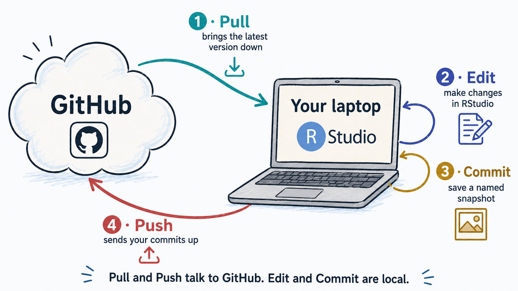
These four moves form a loop you’ll repeat throughout the course. Learn them as a sequence and the rest is detail:
| Move | What it does | When you do it |
|---|---|---|
| Pull | Downloads commits from GitHub and brings them into your local copy | Start of every work session — and any time you’ve been away |
| Edit | Changes files on your computer. Not a Git command — and Git has not recorded anything yet | The bulk of your session |
| Commit | Records the changes you selected, as a labeled checkpoint in your local repository | When you’ve finished a coherent chunk of work — a lab section, a polished figure, anything that “belongs together” |
| Push | Sends your local commits up to GitHub | End of every work session, or any time you want a backup |
The sentence that prevents the most lost work
Only committed changes can be pushed — and saving a file is not committing it. Hitting Cmd/Ctrl + S in RStudio writes your .qmd to your own hard drive and nothing more. It reaches GitHub only after you commit it and then push. If you have ever assumed a file was “backed up because I saved it,” this is the habit to correct now, not the week your laptop dies.
The cycle: pull → edit → commit → push → repeat. Make small commits often. Backup is free; recovery from no backup is not. A natural moment to commit is right after a document renders successfully — that way each snapshot captures not just your latest writing but a working analysis.
Common Git mistake
Don’t wait until the end of the semester to make one giant commit. Commit small pieces as you go — one figure, one section, one cleaned-up lab. Frequent small commits are what make the history useful: each one is a labeled point you can actually return to.
Your first commit · we’ll do this in lab
The hands-on walkthrough of making your first commit and publishing your repository to GitHub happens in the Wednesday M02 lab — with the lab instructor in the room when something doesn’t work. Watching the GitHub Desktop UI for the first time, picking a commit message, deciding what to commit, choosing public vs private — every one of those is a moment where it helps to have someone next to you who’s done it before.
If Git feels more intimidating than the earlier parts of this Module, that’s a very common reaction. For most beginners, Git is the least intuitive tool in the stack at first. The goal for today isn’t mastery; it’s simply to get the software installed and your account connected so that the live walkthrough in lab can focus on the workflow itself.
For today, your job in the version-control section is simpler: install GitHub Desktop, create your GitHub account, and confirm they’re talking to each other. On Wednesday we’ll turn your project into a Git repository, make a first commit, and push it to GitHub — and you’ll leave the lab with a working backup of your course project.
That’s the entire solo workflow: pull → edit → commit → push, repeated over and over. Group projects make the pull-first habit essential (pull to grab teammates’ changes before you edit each session) and add a few conflict-resolution moves — see the callout below for the companion page.
Coming up · Git for group projects
When your project team forms later in the semester, the solo workflow above expands into a collaborative one. Two or three people are now committing to the same repository, and the question of whose changes are where starts to matter. The skills you’ll need to add are:
- Setting up a shared repository — one teammate creates the GitHub repo, invites the others, and everyone clones the repo to their own laptop.
- The pull-first habit — open GitHub Desktop before RStudio every session; pull before you type. This single discipline prevents most conflicts before they happen.
- Coordinating who edits what — divide files or sections among team members so two of you rarely touch the same line of the same file at the same time.
- Resolving conflicts when they happen anyway — what conflict markers look like, how to use RStudio to choose which version stays, and how to commit the resolution.
- Commit-message hygiene — bad commit messages waste your future self’s and teammates’ time; the bar is higher when work is shared.
We’ve collected all of this on a single companion page: Collaborating with Git for group projects. Read it before your first group-project work session. The page also has a daily checklist you can return to every time you sit down to work with teammates.
What NOT to commit
Not every file in your project belongs in version control. Specifically, you should never commit:
- Large, sensitive, or course-distributed data files — especially
.Rds,.csv,.sav,.sas7bdat. These can be many megabytes; Git history bloats fast. Small public example datasets (e.g., a 5-KB CSV that ships with a teaching package) are sometimes committed to real research repositories, but for PSY 652, thedata/folder stays local unless the lab instructor tells you otherwise. - Sensitive data — anything covered by IRB confidentiality, data-use agreements, or personal information you wouldn’t want world-readable. Making a repository private is not the same as making it appropriate for restricted data: do not put IRB-protected, identifiable, or restricted-use data on GitHub — public or private — unless your project has explicit approval and a data-management plan that allows it.
.Rproj.user/— RStudio’s per-user state directory. Different on every machine; commits create noise..Rhistory— R’s per-session history. Personal, not shareable..DS_Store(macOS) andThumbs.db(Windows) — operating-system metadata.- The
output/folder and rendered.htmlfiles — both regenerate from your.qmdsource, so the repository keeps the source instead. (If a workflow of yours genuinely needs rendered files in Git, you can remove those entries; the course default keeps them out.)
Git lets you tell it what to ignore via a special file named .gitignore at the project root. Each line in that file is a pattern describing one or more files Git should leave alone: matching files that are untracked stay out of the staging area, so they are never offered up for a commit. As long as those entries are in .gitignore before you make your first commit — which is how your course project ships — the files they describe simply never enter your repository. (Worth knowing for later: .gitignore does not untrack a file that has already been committed. Once something is in the history, removing it takes an extra step.)
Your project already includes a .gitignore · open it and have a look
Good news — you don’t have to create this file yourself. The PSY652_project/ folder you unzipped earlier this Module already contains a .gitignore at its root, pre-populated for the standard R + Quarto workflow you’ll use all semester. Shipping .gitignore with the project bundle, rather than asking each student to create it, is common professional practice — and it prevents several predictable beginner mistakes. It also avoids two real beginner mistakes: on macOS, files whose names start with a dot (like .gitignore) are hidden by default in Finder; on Windows, Notepad has a habit of silently appending .txt to filenames, which would turn .gitignore into .gitignore.txt and break it without warning.
Open the file in RStudio (in the Files pane, click on .gitignore — RStudio will show it even though Finder may not). You’ll see something like this:
# .gitignore — patterns for files Git should leave untracked. Files NOT matched
# below (your .qmd source, README, codebooks) are eligible to be tracked; they
# reach GitHub only once you commit and push them.

# RStudio per-user state — machine-specific, would only add noise
.Rproj.user/
.Rhistory
.RData
.Ruserdata

# Operating-system junk files
.DS_Store
Thumbs.db

# Data — kept local. Course datasets can be large or restricted, and a private
# repo still isn't a home for protected data. Git tracks code, not data.
data/

# Downloaded source documentation — when a dataset arrives with the provider's
# own codebook, questionnaire, or methodology, file those in a subfolder here
# and they stay local. Your own notes about a source (a flat .md file in this
# folder) are tracked, so the project still records where the data came from.
documentation/*/

# Generated output — regenerates from your .qmd source, so the repo keeps the
# source instead. Delete these two lines only if you need HTML committed.
output/
*.html
The blank lines and lines starting with # are organizational — # introduces a comment, just like in R code. Every other line is one pattern, which can take three forms:
- A literal filename —
.DS_Storeignores every file with exactly that name. - A folder name with a trailing slash —
data/ignores every file inside thedata/folder. This is the line that keeps your NHANES.Rdsfile (and every other course dataset) out of the repo. - A wildcard with
*—*.htmlignores every file whose name ends in.html, regardless of the rest of the name. The asterisk*stands in for “any text here.”
The forms combine, too: documentation/*/ is the wildcard and the trailing slash together, so it reads “any folder inside documentation/.” That is what keeps a provider’s downloaded codebook out of the repo when you file it in its own subfolder — while the .md codebooks sitting loose in documentation/ stay tracked, because they aren’t inside a subfolder. You’ll use this in the M05 lab.
You can edit this file freely. The guiding principle: your source files (.qmd) are what belong in Git; generated files (rendered HTML, anything in output/) do not, because your source can rebuild them. That is why the last two entries are there by default. Some workflows do commit rendered reports — if a course or collaborator ever asks you to submit rendered work through GitHub, delete those two lines. For PSY 652, leave them: finished deliverables go to Canvas, and GitHub holds the source that produced them. Save the file in RStudio after any change; GitHub Desktop will pick it up immediately and the “Changes” list will update.
If you’d rather stay inside RStudio
RStudio has a built-in Git panel (an extra tab in the top-right pane, alongside Environment and History). It does the same four moves — Pull, Commit, Push — and you never have to switch apps. One caveat: that panel only appears when RStudio can find a system Git installation. GitHub Desktop bundles its own Git for its own use, so if GitHub Desktop is all you’ve installed, the RStudio panel may not light up until you install system Git separately. The reasons we recommend GitHub Desktop as the default anyway:
- Cleaner diff view. GitHub Desktop’s side-by-side diff is easier to read for beginners.
- Better conflict UI. When you and a collaborator edit the same file at the same time, GitHub Desktop walks you through resolution; RStudio’s UI assumes you already know what to do.
- The same underlying Git operations. Pulling, committing, pushing, reviewing differences, and resolving conflicts act on the same repository whichever tool you use, so switching later is easy.
If you’ve used Git before and want the in-IDE workflow, RStudio’s panel works fine. For first-timers, start with GitHub Desktop and graduate later.
Looking ahead
This Module is the what of the tool stack — the conceptual map. The hands-on work happens in lab during Week 1, where you’ll bring your laptop and we’ll:
- Verify everything installed correctly — RStudio talks to R, the course packages load, the course project opens.
- Practice the inline-and-rendered workflow — open the lab template, run each chunk, watch the Environment populate, restart R, render to HTML.
- Add a Descriptive Statistics section to the lab template — your first real edit, rendered as polished HTML.
- Turn your project into a Git repository and push it to GitHub — your first commit, your first push, with the lab instructor walking through every click.
The lab is the safety net: if your machine resists any of the install or version-control steps, that’s the right moment to ask for help.
Summary
Core takeaways
The four tools form a single workflow. R is the language, RStudio is the workshop, Quarto is the document system, and Git + GitHub are the version-control layer. None of them stands alone — you’ll touch all four in every lab and every project for the rest of the semester (and, with luck, the rest of your research career).
Local install is the default; Posit Cloud is the safety net. Completing the setup in Week 1 reduces friction for the rest of the semester. Cloud work is a fine safety net, but a local install is usually faster, more flexible, and easier to keep organized. Keep Posit Cloud in your back pocket if a machine refuses to cooperate.
Every analysis you write is a Quarto notebook. A .qmd file mixes prose, code, and the code’s output in one document — render it to produce a clean HTML report that someone can read without R installed. The .qmd is what you maintain; the rendered HTML is the artifact your reader sees.
Project-relative paths and .Rproj files support reproducibility. Opening the project through PSY652_project.Rproj sets RStudio’s working directory to the project folder, so code that uses here::here() runs on your laptop, your collaborator’s, and your future self’s without modification.
Version control is recovery, backup, audit trail, collaboration, and portfolio at once. Make small commits often. Backup is free; recovery from no backup is not. The four moves — pull, edit, commit, push — become muscle memory by Week 3.
Some things do not belong in the PSY 652 repository. Keep the course data/ folder, restricted data, RStudio state files like .Rproj.user/ and .Rhistory, and OS metadata such as .DS_Store out of Git. A starter .gitignore in your project root handles all of these automatically.
The conceptual map is here; the hands-on install is in the M02 lab. Read this Module before Wednesday; the lab is where you bring your laptop, follow the steps with the lab instructor present, and leave with a verified-working stack.
Resources
Learning the toolchain takes time, and there are excellent free resources to lean on as questions come up:
- R for Data Science (Wickham, Çetinkaya-Rundel, & Grolemund) — the canonical introduction to R + tidyverse + Quarto. Available free at r4ds.hadley.nz.
- Happy Git with R (Bryan & The STAT 545 TAs) — the gentlest possible introduction to Git, GitHub, and the RStudio Git workflow. happygitwithr.com.
- Quarto documentation — every feature, with examples. quarto.org/docs.
- The Posit Community Forum — well-moderated, beginner-friendly. forum.posit.co.
- GitHub Docs · GitHub Desktop — short, focused articles on every Desktop feature. docs.github.com/desktop.
Footnotes
Here
foois programmer shorthand for “any name at all” — a generic stand-in, the way “so-and-so” stands in for an unnamed person. It isn’t a special Quarto word; it just means whatever your file happens to be called. Sofoo.qmd→foo.htmlis the general rule, andm02_lab.qmd→m02_lab.htmlorlab_template.qmd→lab_template.htmlare two specific cases of it.↩︎Throughout this Module,
Cmd/Ctrlmeans “useCmd(⌘) on macOS, orCtrlon Windows and Linux” for the shortcut being described. Mac keyboards do also have a Control key — it simply isn’t the equivalent key in these particular shortcuts. (And every keyboard shortcut in this Module also has a menu or on-screen-button equivalent, so you never have to memorize one. If a chord doesn’t work on your machine, look it up under Tools → Keyboard Shortcuts Help, which shows the bindings your installation actually uses.)↩︎