library(tidyverse)
library(here)
library(broom)
library(effectsize)
library(infer)Simple Linear Regression
Learning Objectives
By the end of this Module, you should be able to:
The line and its geometry
- Explain the purpose of simple linear regression (SLR) for modeling the relationship between two variables.
- Distinguish a deterministic relationship from a statistical (probabilistic) model, and explain the role of the residual.
- Evaluate whether a straight-line summary is appropriate for a pair of variables (linearity check).
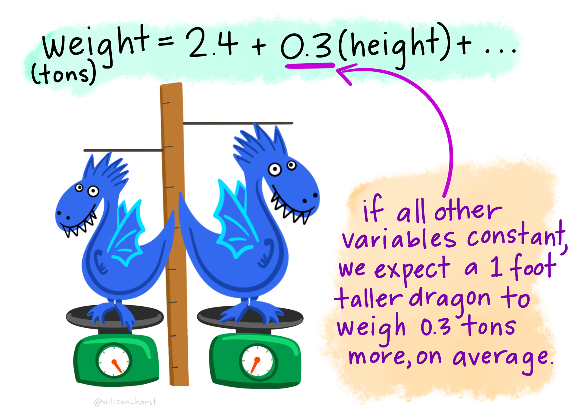
- Interpret the intercept (\(b_0\)) and slope (\(b_1\)) of a regression line in applied terms.
- Define and compute a predicted value (\(\hat{y}_i\)) and a residual (\(e_i\)) by hand.
- State the least squares criterion and explain why it defines the best-fitting line.
- Explain why centering a predictor changes the intercept’s meaning but not the slope, and recognize regression toward the mean as a statistical pattern rather than evidence that anyone changed.
Fitting and reading the model in R
- Fit a simple linear regression with lm(), and extract output via tidy(), glance(), and augment().
- Interpret R² as the proportion of variance in \(Y\) explained by \(X\), and \(\sigma\) (the residual standard error) as the typical scale of residual error in the outcome’s units.
- Distinguish the unstandardized slope from the correlation coefficient \(r\), and recognize that \(r^2 = R^2\).
- Quantify the uncertainty in a slope — its standard error, \(t_\text{obs}\), confidence interval, and p-value — by formula and by bootstrap, and explain why the slope’s t-test and the F-test agree in SLR.
- Distinguish a confidence interval for the regression line from a prediction interval for a new observation.
Categorical predictors and the bridge back to M09
- Use a binary categorical predictor in regression: read contrasts(), interpret the intercept as the reference-group mean and the slope as a between-group mean difference.
- Use a multi-category categorical predictor: anticipate the \(k - 1\) dummy variables R will create, recover group means from the coefficients, visualize the five contrasts, compute each contrast’s \(t_\text{obs}\), p-value, and CI, and tell those five separate tests from the omnibus F-test.
- Connect the categorical-predictor regressions to the two-sample t (M09 Test 1) and the one-way ANOVA (M09 Test 2): same numbers, different framing — and compute Cohen’s d from the regression’s mean difference.
- Report simple linear regression results in APA style, with coefficients, CIs, R², and \(\sigma\).
Overview
Where this fits — the Part 3 regression arc
Part 2 gave you different tools for different designs: a t-test for two groups, ANOVA for several groups, and chi-square for a table of counts. Part 3 shifts from that collection of separate tests to a single modeling framework: regression. A regression model describes how the average outcome varies with one or more predictors.
This framework reaches backward and forward. Looking backward, the two-sample t-test and one-way ANOVA from M09 turn out to be special cases of the linear model. Looking forward, the same framework can accommodate several predictors at once — for example, adjusting a treatment comparison for where participants started or for other measured differences between them. And the core ideas you learn here — coefficients, predictions, residuals, estimands, and model checking — carry into many of the more advanced models you’ll meet later, including logistic, multilevel, and structural equation models.
With a model as the tool, the workflow becomes fit → query → check. Modules 10–12 take one step each, all using the REACH forgiveness trial you met in the Part 2 lectures:
- M10 · Fit — What relationship does the model estimate? (slopes, intercepts, residuals, fit) · ← you are here
- M11 · Query — What adjusted estimand answers the research question? (partial effects, adjusted comparisons)
- M12 · Check — Are the model’s assumptions good enough to trust the inference? (diagnostics, remediation)
One workflow, three verbs: fit the model → query it for the estimand you care about → check that it’s trustworthy enough to report. That workflow carries forward into the more advanced models you’ll meet as you go further. The models become more sophisticated; the basic way of thinking stays the same.
Imagine you’ve just helped run a randomized controlled trial for a forgiveness intervention. For every participant you have two benevolence scores — one before, one two weeks after — plus which of six study sites they came from and whether they received the workbook or waited for it. Your advisor wants answers by Friday, and each question she asks turns out to be about the size and shape of a relationship: not whether two things are related, but how much, in what direction, and how sure you can be.
In M07–M09 we built the toolkit for asking is there a difference? — confidence intervals around a mean, hypothesis tests on a single mean, on two means, on three or more means, on a categorical 2×2 table. Those tools answered questions about specific means and group contrasts.
Most research questions in applied psychology go beyond asking simply whether something is related to something else. We usually want to know how much, in what direction, for whom, and after accounting for what else. Questions like:
- How strongly does baseline benevolence predict benevolence two weeks later? How much higher is predicted T2 benevolence for people who start one point higher on T1 benevolence?
- How well can we predict someone’s follow-up benevolence from what we know about them at baseline?
- Does random assignment to the REACH workbook produce higher follow-up benevolence than waitlist control — and by how much?
- Does that treatment difference remain after accounting for baseline benevolence and other relevant covariates?
- Does the effect of the workbook differ as a function of baseline benevolence or across the six study sites — and if so, by how much?
- What are the mechanisms of change? Does the workbook raise benevolence by reducing revenge motivations, increasing empathy, or both?
- How much of the variation in an outcome can the predictors in our model account for, and how much remains unexplained?
Regression supplies the modeling framework behind many of these analyses. It turns relationships, group differences, predictions, and adjusted comparisons into quantities we can estimate, attach uncertainty to, and interpret in the language of the research question. Some of these questions, especially causal mechanisms, mediation, and differences in treatment effects, need additional design and identification assumptions beyond fitting a regression equation.
This Module builds the simplest version of regression — simple linear regression (SLR), with one outcome and one predictor variable — and applies it three times, with the predictor each time being a different kind of variable:
- A continuous predictor (T1 benevolence → T2 benevolence, restricted to Hong Kong control participants).
- A binary categorical predictor (treatment condition → T2 benevolence) — the dummy-coding case.
- A multi-category categorical predictor (study site → T1 benevolence) — the multi-dummy case.
Three passes, one framework
- Continuous predictor → learn the geometry of a regression line: slope, intercept, residuals, fit.
- Binary predictor → watch regression reproduce a two-group mean difference (M09’s two-sample t).
- Multi-category predictor → watch it reproduce the one-way ANOVA (M09 Test 2).
The same few lines of code run all three — lm(), tidy(), and glance(), with augment() whenever you need fitted values and residuals. All that changes is the kind of predictor on the right of the ~.
In Parts 2 and 3 of this Module, you’ll see that two of M09’s tests — the two-sample t (Test 1) and the one-way ANOVA (Test 2) — are special cases of regression. That’s not coincidence; it’s the regression-as-parent-framework point M09’s Looking ahead section previewed. M11 will then layer predictors on top of each other to ask compound questions. And, in PSY 653, you’ll see that the same framework can accommodate more complex designs, including mediation, moderation, and multilevel designs.
Packages used in this module
Meet the data
This Module’s examples all use a single research context — the REACH Forgiveness intervention study (Ho et al., 2024, BMJ Public Health · PDF).
The REACH study
REACH was a multisite randomized waitlist-controlled trial of a self-directed forgiveness workbook, conducted at six sites in five countries (Colombia, Hong Kong, Indonesia, South Africa, and Ukraine) between February 2020 and October 2021. N = 4,598 adults aged 18 and older, each of whom had experienced an interpersonal transgression and was asked to recall someone who had “deeply hurt or offended” them. Median age 26, 73–75% female (by arm), 87% with secondary education or higher, 76–77% religiously affiliated (Ho et al., 2024, Table 1).
Participants were randomly assigned to receive the workbook immediately (treatment, n = 2,290) or after a 2-week delay (waitlist control, n = 2,308); randomization was done within each site. Course analyses use baseline (T1, pre-randomization) and the 2-week follow-up (T2). The dataset has six site values. Ukraine has two collection sites: UISA (the paper’s “Ukraine site 1”: university students plus members of a Christian church) and Realis (“Ukraine site 2”: members of a Christian church). The single Colombia value combines two subsites, university students and survivors of war. treat is approximately balanced, both overall and within each site.
The intervention is a 2–3 hour self-directed workbook based on the REACH Forgiveness program (originally created by Dr. Everett Worthington). REACH is the acronym:
- R — Recall the hurt
- E — Empathize with the offender
- A — Give an Altruistic gift of forgiveness
- C — Commit to the forgiveness experienced
- H — Hold onto forgiveness
The trial had three primary outcomes: unforgiveness, depression symptoms, and anxiety symptoms. Unforgiveness was measured with the TRIM-18 (Transgression-Related Interpersonal Motivations Inventory) — eighteen 1–5 Likert items tapping three motivations toward the person who caused the hurt. The authors reverse-scored the benevolence items and combined all 18 items into a single unforgiveness score. In our data file, the items are ordered by subscale (the published questionnaire mixes them):
| Items (our file) | Subscale | Direction |
|---|---|---|
| 1–5 | Revenge motivations — desire to seek harm to the offender | higher = more unforgiving |
| 6–12 | Avoidance motivations — desire to withdraw from the offender | higher = more unforgiving |
| 13–18 | Benevolence motivations — positive goodwill toward the offender | higher = more forgiving |
For this Module we use benevolence on its own — the average of items 13 through 18 at each timepoint. That is a course choice, not the paper’s outcome, so our estimates are not the paper’s. Higher benevolence means more forgiveness; the intervention is designed to raise it.
reach_analysis · 4,598 participants · 6 sites × 2 conditions · between-subjects RCT · Ho et al. (2024)
The course-prepared subset of Ho et al. (2024). One row per participant; T1 and T2 in separate columns. Available at data/reach_analysis.Rds.
uid integer — Unique participant identifier
site factor — Which of six international study sites the participant was recruited at
treat factor — Randomized condition: the REACH forgiveness workbook intervention, or waitlist control
age numeric — Age in years at baseline
t1_trim1 numeric — TRIM-18 item at baseline
t2_trim1 numeric — TRIM-18 item at follow-up
t1_benevolence numeric — Benevolence subscale of the TRIM-18 at baseline, the mean of t1_trim13; t1_trim14; t1_trim15; t1_trim16; t1_trim17; t1_trim18
t2_benevolence numeric — Benevolence subscale of the TRIM-18 at follow-up, the mean of t2_trim13; t2_trim14; t2_trim15; t2_trim16; t2_trim17; t2_trim18
t1_revenge numeric — Revenge subscale of the TRIM-18 at baseline, the mean of t1_trim1; t1_trim2; t1_trim3; t1_trim4; t1_trim5
t2_revenge numeric — Revenge subscale of the TRIM-18 at follow-up, the mean of t2_trim1; t2_trim2; t2_trim3; t2_trim4; t2_trim5
Plus demographic columns (sex, eth, educ, income, hasReligAffil, maritalStat) — held in reserve for later Modules.
This Module’s three regressions all run on the benevolence subscale. Another of the instrument’s subscales — revenge motivations (t1_revenge / t2_revenge, TRIM items 1–5 in our file) — is in the file too, but M10 doesn’t analyze it. Because it’s scored so that higher means more vengeful, a treatment contrast on revenge would carry the opposite sign from the one on benevolence.
Full codebook for reach_analysis — values, levels, missingness, and how the file was prepared.
Want to see how this dataset was built?
The cleaning, demographic re-coding, TRIM-18 reverse-coding, subscale construction, and reliability checks all live in a public Posit Cloud project: psy652-reach-data-prep. A (free) Posit Cloud account is required. Open it any time you want to see the data-processing layer that comes before the analyses we run in this Module.
reach <- read_rds(here("data", "reach_analysis.Rds"))reach |>
select(uid, site, treat, t1_benevolence, t2_benevolence) |>
glimpse()Rows: 4,598
Columns: 5
$ uid <int> 1, 2, 3, 4, 5, 6, 7, 8, 9, 10, 11, 12, 13, 14, 15, 16, …
$ site <fct> Hong Kong, Hong Kong, Hong Kong, Hong Kong, Hong Kong, …
$ treat <fct> Control, Treatment, Treatment, Treatment, Treatment, Co…
$ t1_benevolence <dbl> 2.666667, 3.666667, 4.333333, 4.000000, 3.000000, 2.333…
$ t2_benevolence <dbl> 2.833333, 3.000000, 5.000000, 4.000000, 3.666667, 2.333…Some participants — about 14% — are missing T2 benevolence (lost to the 2-week follow-up). For analyses with t2_benevolence as the outcome (Parts 1 and 2 of this Module), we’ll drop those rows via drop_na() — an approach called listwise deletion (or complete-case analysis); for the Part 3 analysis on baseline benevolence (t1_benevolence), we keep the full sample.
reach |>
  summarize(
    n_total = n(),
    n_with_t1 = sum(!is.na(t1_benevolence)),
    n_with_t2 = sum(!is.na(t2_benevolence)),
    M_t1 = mean(t1_benevolence, na.rm = TRUE) |> round(2),
    SD_t1 = sd(t1_benevolence, na.rm = TRUE)   |> round(2),
    M_t2 = mean(t2_benevolence, na.rm = TRUE) |> round(2),
    SD_t2 = sd(t2_benevolence, na.rm = TRUE)   |> round(2)
  )
Listwise deletion — and the special risk in a randomized trial. Here we drop follow-up non-completers with drop_na() — listwise deletion (a.k.a. complete-case analysis), PSY 652’s default throughout. M05 (Describing Data with R) laid out its general trade-offs. Complete-case analysis always loses information, and so power and precision: every dropped row shrinks the effective n, which tends to widen CIs. It can also introduce bias when whether a participant has a follow-up score is related to the outcome in ways the analysis doesn’t account for. Data missing completely at random (MCAR) protect against that bias, but MCAR is one simple condition that does so, not the only one. One version of that bias deserves special attention here, because REACH is a randomized trial: differential attrition. Randomization makes the two arms comparable at the moment of assignment — but it guarantees nothing about who stays. If, within an arm, whether someone completes the follow-up is related to their benevolence (say, the workbook’s least-helped participants lose interest while controls stay regardless), complete-case analysis quietly unbalances the very comparison randomization was built to protect, and the treatment-effect estimate inherits that bias. Different dropout rates alone don’t create this bias; dropout that is related to the outcome does. The principled fixes — multiple imputation and FIML — and the full toolkit are M05’s story, and more advanced courses develop them in depth. For now: use drop_na(), name it as listwise deletion, and in a trial, always report attrition by arm.
Part 1 — A continuous predictor
What kind of question is this? Part 1 is associational/predictive, not causal. We’re asking how baseline benevolence forecasts follow-up benevolence within a single arm — there’s no intervention, no random-assignment manipulation; we’re just describing the test–retest relationship. Part 2 will be the causal part of the Module (because of REACH’s random assignment to treatment); Part 3 will be descriptive, comparing pre-treatment baselines across study sites.
Our first regression asks: In the absence of any intervention, how predictable is post-test benevolence from pre-test benevolence?
To build intuition cleanly, we’ll work through Part 1 with a single site — the Hong Kong control arm (n = 173). The full REACH sample has 4,598 participants, which is wonderful for precise estimation but produces visualizations so dense that the conceptual steps we want to highlight — how much a regression line can wiggle from sample to sample, where residuals sit relative to the line, how a confidence band fans out at the extremes — become hard to see. The Hong Kong control arm is small enough to show the geometry clearly, but still real data with everything we need. Once the concepts are anchored, Part 2 expands to both arms and all six sites to ask a benevolence version of the treatment-effect question REACH was built to answer.
Restricting to the control arm is also deliberate. The control group received no workbook during the 2-week interval, so any T1-to-T2 association we see reflects natural test–retest stability — the degree to which someone’s baseline forgiveness disposition forecasts their disposition two weeks later, in the absence of intervention. That’s a much cleaner setup for first-exposure regression than mixing it with an active treatment.
control <- reach |>
  filter(treat == "Control", site == "Hong Kong") |>
  drop_na(t1_benevolence, t2_benevolence)

control |>
  summarize(
    n = n(),
    M_x = mean(t1_benevolence) |> round(2),
    SD_x = sd(t1_benevolence)  |> round(2),
    M_y = mean(t2_benevolence) |> round(2),
    SD_y = sd(t2_benevolence)  |> round(2)
  )
The sample has 173 Hong Kong control participants with both timepoints. Mean baseline benevolence is 3.05 (SD = 0.88); mean follow-up benevolence is 3.03 (SD = 0.80). On a 1–5 scale, both averages sit just above the midpoint, and they are nearly identical: the T1→T2 change in the mean (-0.02) shows that, in this Hong Kong control arm, with no workbook, average benevolence barely moves over two weeks.
Deterministic relationships vs statistical models
Before we draw a line through the scatter, let’s build the right intuition for what kind of model we’re fitting. The key distinction is between a relationship that determines an outcome exactly and one that describes what tends to happen on average.
A deterministic relationship gives the same outcome every time the input is known. The perimeter of a square is \(4 \times s\). The area of a circle is \(\pi r^2\). Once you know the input, the rule determines the output exactly.
A statistical model is different. Knowing \(X\) helps us predict \(Y\), but it usually doesn’t determine \(Y\) perfectly. Real outcomes vary because we haven’t measured every relevant predictor, our measurements contain error, and people (or schools, or experimental subjects) differ in ways the model doesn’t capture. A statistical model therefore separates the outcome into two pieces:
\[\text{Outcome} \;=\; \underbrace{\text{Systematic component}}_{\text{what the model predicts}} \;+\; \underbrace{\text{Residual}}_{\text{what remains}}\]
In regression, the systematic component is the value predicted by the fitted line. The residual is the difference between a person’s observed outcome and that prediction. Fitting a regression line therefore does not claim that \(X\) determines \(Y\). It says that \(X\) helps us describe the average pattern in \(Y\), while individual observations still vary around that pattern.
Two different kinds of relationship
| Deterministic relationship | Statistical model | |
|---|---|---|
| Form | \(y = f(x)\) | \(y_i = f(x_i) + e_i\) |
| Once \(x\) is known… | \(y\) is determined exactly | \(y\) can still vary |
| Residual term? | No | Yes |
| Example | Geometry, conversion formulas | Most data in psychology, education, and public health |
The regression models in this course are statistical models: they describe systematic patterns while explicitly allowing observations to vary around those patterns.
Looking at the data
Our first research question is: How does baseline benevolence predict 2-week follow-up benevolence? As always, starting with a visual inspection of the data is a good idea. A scatterplot is the right first step. Here we will map T1 benevolence onto the x-axis (predictor) and T2 benevolence onto the y-axis (outcome):
Show the code that built this figure
control |>
  ggplot(aes(x = t1_benevolence, y = t2_benevolence)) +
  geom_jitter(width = 0.05, height = 0.05, alpha = 0.35,
              color = "#3A8055", size = 1.4) +
  scale_x_continuous(breaks = 1:5) +
  scale_y_continuous(breaks = 1:5) +
  labs(
    x = "T1 benevolence (1–5)",
    y = "T2 benevolence (1–5)",
    title = "Hong Kong control arm — benevolence: T1 vs T2",
    subtitle = paste0("n = ", nrow(control), " participants. \nSmall jitter added so overlapping respondents are visible.")
  )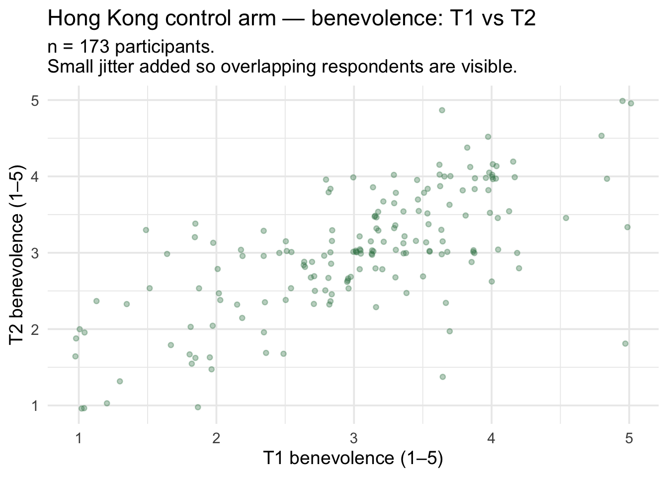
The cloud rises from lower-left to upper-right: people who started higher in benevolence tend to end higher; people who started lower tend to end lower. There’s substantial spread — at any value of T1 there are many T2 values — so the relationship is not deterministic, but it’s clearly there.
Is the relationship linear?
Before we summarize this scatter with a straight line, we have to decide whether a straight-line summary is appropriate. A straight line says two people one unit apart on \(X\) are predicted to differ by the same amount on \(Y\), wherever on the \(X\) scale they sit. That’s a strong assumption — many real-world relationships are curved.
Here are four curved shapes you might encounter: a U, an inverted U, exponential growth, and a logarithmic curve that rises quickly and then levels off.
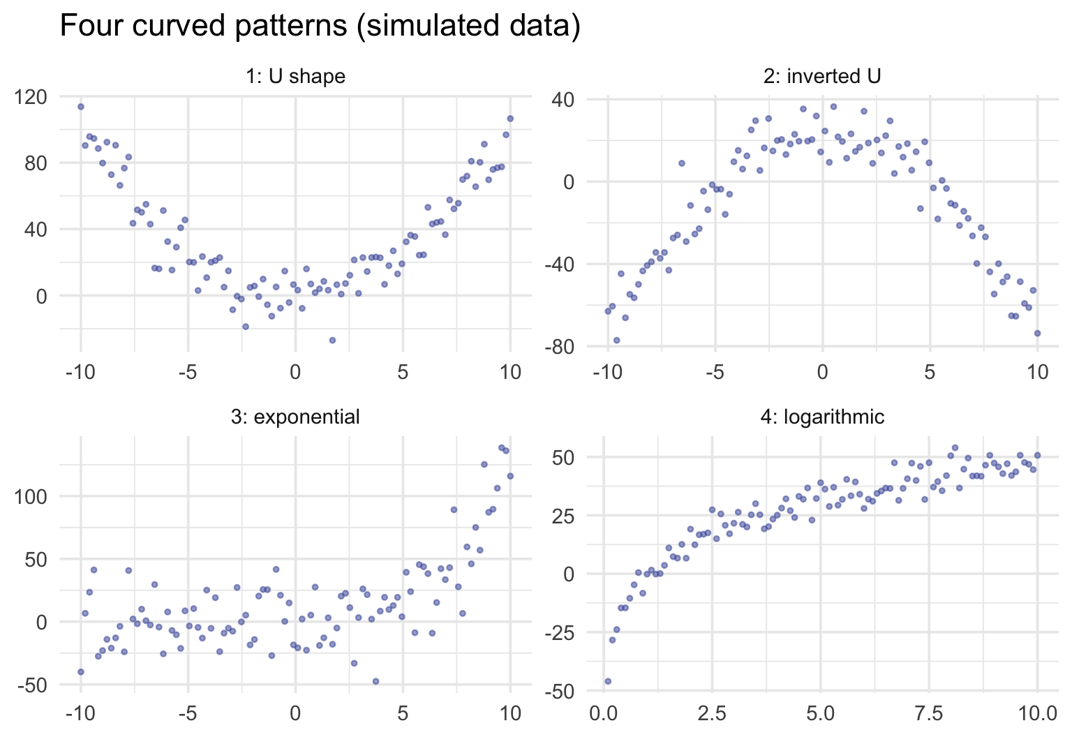
Curves differ in how much a straight line misses. For the U and the inverted U, a single line can miss the pattern almost entirely: its slope can sit near zero even though \(Y\) depends strongly on \(X\). For curves that keep rising, like the exponential and the logarithmic, a line still describes the average trend, but it hides the bend, so its predictions run systematically high in some ranges of \(X\) and low in others. As Gelman, Hill, and Vehtari put it in Regression and Other Stories, “just about every problem we ever study will be nonlinear, but linear regression can still be useful in estimating an average relationship.” When the bend matters for your question, regression is still the tool: a transformation (log, square root) or a polynomial term lets a regression model follow a curve. M12 shows how to check for curvature, and more advanced courses take up those models.
For our Hong Kong scatter, the cloud rises at a roughly steady rate across the whole 1–5 baseline range — no obvious bend, no flattening at the extremes. A straight line is a reasonable summary. Here’s the ordinary least squares (OLS) line overlaid — least squares is the fitting rule we define carefully a few sections below; for now, read “OLS line” as “the best-fitting straight line through the cloud of data points”:
control |>
  ggplot(aes(x = t1_benevolence, y = t2_benevolence)) +
  geom_jitter(width = 0.05, height = 0.05, alpha = 0.35,
              color = "#3A8055", size = 1.4) +
  geom_smooth(method = "lm", formula = y ~ x, se = FALSE,
              color = "#C05852", linewidth = 1.2) +
  scale_x_continuous(breaks = 1:5) +
  scale_y_continuous(breaks = 1:5) +
  labs(
    x = "T1 benevolence (1–5)",
    y = "T2 benevolence (1–5)",
    title = "Hong Kong control arm — T1 vs T2 with OLS line",
    subtitle = "The rose line minimizes the sum of squared vertical residuals — see below."
  )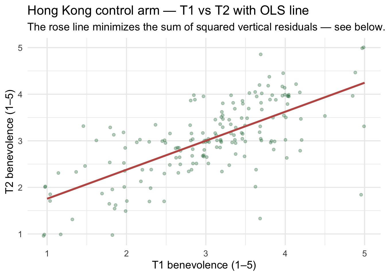
The line summarizes the relationship: comparing people one point apart on T1, the line predicts their T2 scores differ by some fraction of a point. The rest of this section unpacks what that fraction is, how it gets computed, and how to communicate it.
The intercept and the slope
A regression line is defined by two numbers — the intercept \(b_0\) and the slope \(b_1\):
\[\hat{y}_i \;=\; b_0 \;+\; b_1 \cdot x_i\]
- Intercept \(b_0\) — the predicted value of \(y\) when \(x = 0\). On our chart, that’s where the line crosses the y-axis.
- Slope \(b_1\) — the predicted difference in \(y\) between two people whose \(x\) values differ by one unit. On our chart, that’s the rise of the line per one unit of run.
Why “a difference between people” rather than “a change in a person”? Our data compare different participants who happened to have different baseline scores; nobody’s baseline was changed. So the slope describes how people with different T1 scores differ, on average, at T2. That is a comparison between people, which Gelman, Hill, and Vehtari call “the safest interpretation of a regression.” Reading the slope as what would happen if one person’s T1 went up by a point is a within-person, causal claim, and these data can’t support it on their own. (When the predictor is randomly assigned, as treatment is in Part 2, the comparison can support a causal reading.)
The hat (\(\hat{y}\)) signals “predicted from the model” rather than “observed in the data.” For each participant \(i\), \(\hat{y}_i\) is what the line predicts (e.g., for T2 benevolence) given that participant’s \(x_i\) score (e.g., T1 benevolence); the gap between \(\hat{y}_i\) and the actual \(y_i\) is the residual \(e_i = y_i - \hat{y}_i\).
Rearranging that definition gives the full model for each observation:
\[y_i \;=\; \underbrace{b_0 \;+\; b_1 x_i}_{\text{the line (systematic part)}} \;+\; \underbrace{e_i}_{\text{the residual}}\]
Each person’s observed score is the line’s prediction for them plus their own residual. This is the statistical model from the start of this Part, now written with the regression line: outcome = systematic component + residual.
Visualizing the intercept
The intercept is the line’s height at \(x = 0\). The 1–5 benevolence scale doesn’t include 0, so the intercept is technically an extrapolation beyond the data — but it’s still where the math says the line crosses. Here it’s marked in rose at the y-axis:
Show the code that built this figure
ctrl_mod_for_demo <- lm(t2_benevolence ~ t1_benevolence, data = control)
b0_demo <- ctrl_mod_for_demo |> coef() |> pluck("(Intercept)")
b1_demo <- ctrl_mod_for_demo |> coef() |> pluck("t1_benevolence")

control |>
  ggplot(aes(x = t1_benevolence, y = t2_benevolence)) +
  geom_jitter(width = 0.05, height = 0.05, alpha = 0.30,
              color = "#3A8055", size = 1.4) +
  geom_abline(intercept = b0_demo, slope = b1_demo,
              color = "#C05852", linewidth = 1.2) +
  geom_point(aes(x = 0, y = b0_demo), inherit.aes = FALSE,
             color = "#C05852", size = 4) +
  annotate("label", x = 0.4, y = b0_demo + 0.25,
           label = sprintf("intercept = %.3f", b0_demo),
           color = "#C05852", fontface = "bold", fill = "white",
           label.size = 0, hjust = 0) +
  scale_x_continuous(breaks = 0:5) +
  scale_y_continuous(breaks = 0:5) +
  labs(
    x = "T1 benevolence (1–5)", y = "T2 benevolence (1–5)",
    title = "The intercept of the regression line",
    subtitle = paste0("At x = 0, the model predicts ŷ = ", sprintf("%.3f", b0_demo), ".\n",
                      "x = 0 is outside the 1–5 scale, so interpret with caution.")
  )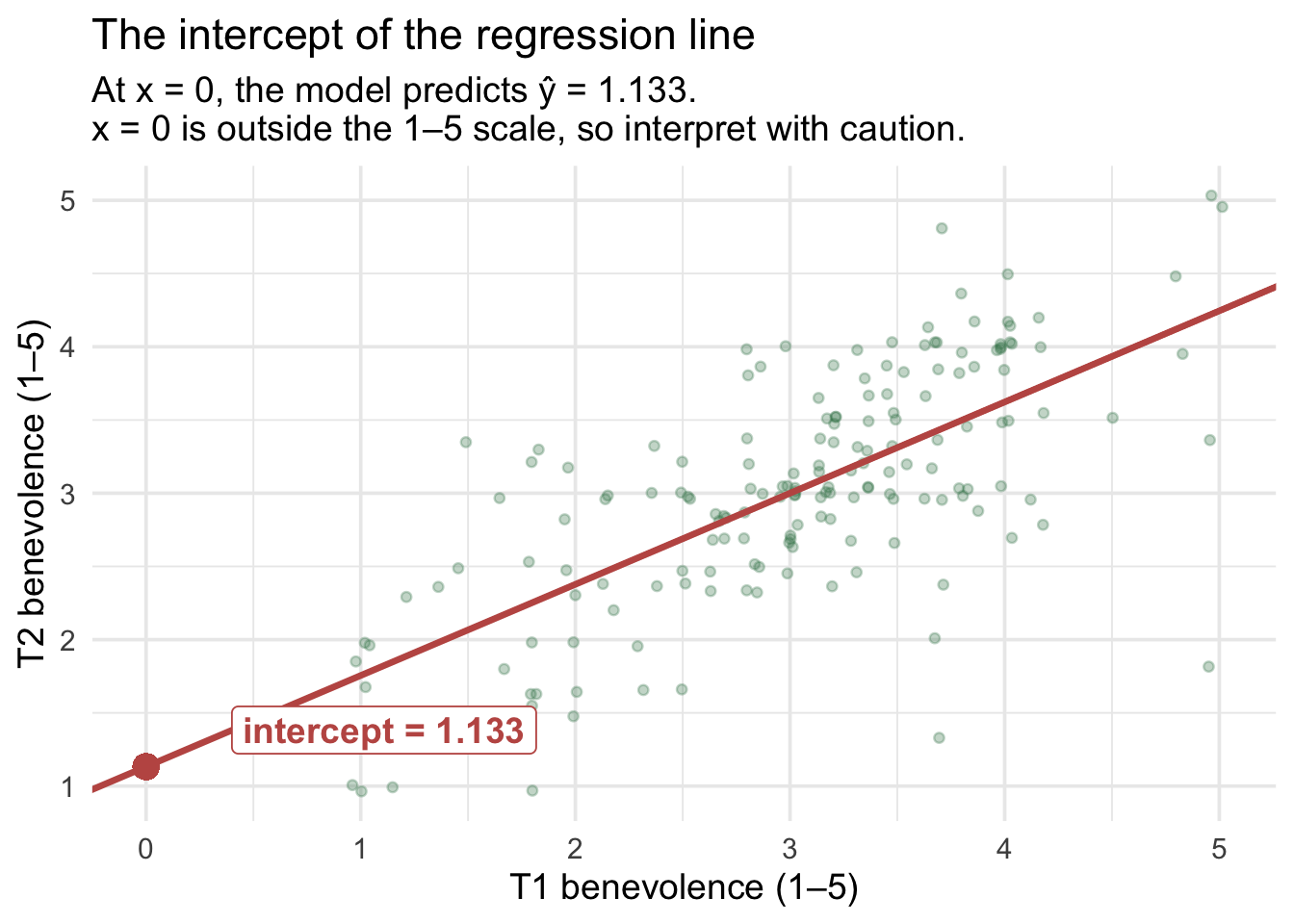
This particular intercept of 1.133 is a mathematical extrapolation: the data don’t include anyone with T1 = 0. A few sections below — Centering: when zero isn’t a useful baseline — we’ll see how re-expressing the same model with a shifted zero (a reparameterization) makes the intercept land at a value that is in the data, with a much friendlier interpretation.
Visualizing the slope
The slope is the rise per unit run. On our line, here’s the rise from \(x = 2\) to \(x = 3\):
Show the code that built this figure
x1 <- 2; x2 <- 3
y1 <- b0_demo + b1_demo * x1
y2 <- b0_demo + b1_demo * x2

control |>
  ggplot(aes(x = t1_benevolence, y = t2_benevolence)) +
  geom_jitter(width = 0.05, height = 0.05, alpha = 0.30,
              color = "#3A8055", size = 1.4) +
  # The 45-degree identity line (T2 = T1), for comparison with the fitted slope
  geom_abline(intercept = 0, slope = 1,
              color = "grey55", linewidth = 0.7, linetype = "dotted") +
  annotate("label", x = 4.65, y = 4.85, label = "T2 = T1 line",
           color = "grey40", size = 3.1, fill = "white", label.size = 0) +
  geom_abline(intercept = b0_demo, slope = b1_demo,
              color = "#C05852", linewidth = 1.2) +
  annotate("segment", x = x1, xend = x2, y = y1, yend = y1,
           color = "#C05852", linewidth = 1.4, linetype = "dashed") +
  annotate("segment", x = x2, xend = x2, y = y1, yend = y2,
           color = "#C05852", linewidth = 1.4, linetype = "dashed") +
  annotate("label", x = (x1 + x2)/2, y = y1 - 0.32,
           label = "run = 1 unit", color = "#C05852",
           fontface = "bold", fill = "white", label.size = 0) +
  annotate("label", x = x2 + 0.18, y = (y1 + y2)/2,
           label = sprintf("rise = %.3f", y2 - y1), color = "#C05852",
           fontface = "bold", fill = "white", label.size = 0, hjust = 0) +
  scale_x_continuous(breaks = 1:5) +
  scale_y_continuous(breaks = 1:5) +
  labs(
    x = "T1 benevolence (1–5)", y = "T2 benevolence (1–5)",
    title = "The slope of the regression line",
    subtitle = sprintf("Participants 1 point apart on T1 are predicted to differ by %.3f on T2.", b1_demo)
  )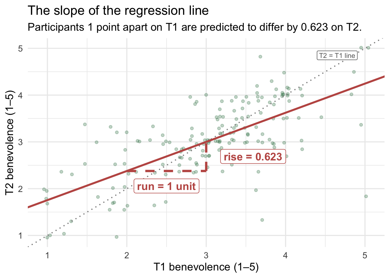
Compare two participants whose T1 scores differ by one point: the model predicts their T2 scores differ by 0.623 points. Notice this is less than 1. The dotted gray line in the figure is the identity line — where every point would sit if everyone’s T2 exactly equaled their T1 — and the fitted rose line is visibly shallower than it: low T1 scorers are predicted to land above their baseline, high T1 scorers below it. That tilt-toward-the-middle has a name, and a deep statistical explanation. The next subsection takes it on directly.
Regression toward the mean: a statistical pattern, not necessarily a process
Because T1 and T2 use the same scale and have similar means and SDs here, the shallow raw slope (0.623 rather than 1.000) gives an intuitive preview of a phenomenon called regression toward the mean (RTM). The clean mathematical version appears on the standardized scale below, \(\widehat{z}_{T2} = r\,z_{T1}\). Put simply: observations that are unusually extreme on one measurement tend, on average, to be less extreme on a later measurement, whenever the two measurements are less than perfectly associated. That is a statement about the average for a group selected because its first scores were extreme. It does not mean every extreme individual moves toward the mean; some become even more extreme. The control arm of REACH received no workbook during those two weeks; yet our model predicts that participants who scored a 5 on benevolence at T1 will, on average, score about 4.25 at T2 — not a 5 again. The pull toward the average is noticeable.
Crucially: this pattern is not, by itself, evidence that people psychologically changed toward the average. No one is necessarily “becoming less benevolent” because they used to be very benevolent; the pattern appears even when nothing about the person changed. (Genuine change can occur alongside regression toward the mean — the point is that RTM alone is enough to produce the pattern.) The standardized view below shows the pattern exactly; the folded box after it explains one common reason it happens.
Correlation gives the cleanest picture of the regression
Regression toward the mean is easiest to see when both measurements are expressed in standard-deviation units. Suppose a participant’s T1 score is \(z_{T1}\) standard deviations above or below the T1 mean. In simple linear regression, their predicted standardized T2 score is
\[\widehat{z}_{T2} \;=\; r \, z_{T1}\]
That equation makes the phenomenon visible immediately:
- If \(r = 1\), an observation 2 SDs above the T1 mean is predicted to remain 2 SDs above the T2 mean. There is no regression toward the mean.
- If \(r = .60\), an observation 2 SDs above the T1 mean is predicted to be only \(2 \times .60 = 1.20\) SDs above the T2 mean.
- If \(r = 0\), knowing T1 tells us nothing about T2, so every person’s predicted T2 score is simply the T2 mean.
When two measurements are positively but imperfectly correlated, the smaller the correlation, the stronger the predicted regression toward the mean. At a correlation of 1, there is no regression toward the mean in standardized units; as the correlation approaches 0, predicted scores move closer to the second measurement’s mean. For the Hong Kong control arm, \(r\) = .69.
Why not simply use our raw regression slope? Because
\[b_1 \;=\; r \times \frac{SD_{T2}}{SD_{T1}}\]
so the unstandardized slope depends not only on the strength of the association but also on the relative spreads of T1 and T2. In our data, both occasions use the same 1–5 benevolence scale, and their SDs are similar but not identical (0.88 at T1, 0.80 at T2), so \(b_1\) = 0.62 sits a little below \(r\). The raw slope still gives a reasonable visual picture of the shrinkage in benevolence points: roughly 62% of a deviation from the average T1 is carried forward to T2. (Because benevolence is bounded at 1 and 5, ceiling and floor effects can intensify the pattern at the extremes: scores near the boundaries have less room to move farther out than in.) In general, though, \(r\) is the cleaner, scale-free way to understand regression toward the mean.
The predictions regress far more than the group does. It’s tempting to read a slope below 1 as a sign that the whole group is converging, with everyone’s scores bunching toward the middle over two weeks. The data say otherwise. T2 is nearly as spread out as T1 (SD = 0.80 at T2 vs 0.88 at T1), while the model’s predictions are much less spread out (SD = 0.55). Each prediction is pulled toward the mean, because the two occasions are imperfectly correlated. But each participant’s actual T2 score is their prediction plus their own residual, and the residuals add the spread back. Reading regression toward the mean as evidence that a group is converging, or that its extreme members changed, is a well-known mistake called the regression fallacy. A classic example from psychology, reported by Tversky and Kahneman: flight instructors noticed that an excellent maneuver was usually followed by a worse one, and concluded that praising trainees hurt their performance. Regression toward the mean predicts exactly that pattern even if praise has no effect at all.
Here \(r\) also describes the test–retest stability of benevolence across the two occasions. A strong test–retest correlation can reflect reliable measurement, stable individual differences, or both, so it shouldn’t automatically be read as a pure estimate of measurement reliability. We’ll return to this relationship later in the Module, when we standardize both variables and see that the standardized regression slope is exactly \(r\).
TipGoing further — why RTM happens, and where the name comes from
A two-component intuition. Imagine that any participant’s observed benevolence score on a given occasion is the sum of two pieces:
\[\underbrace{\text{observed score at T1}}_{y_{T1}} \;=\; \underbrace{\text{true level of benevolence}}_{\text{the stable part}} \;+\; \underbrace{\text{transient noise on that day}}_{\text{the random part}}\]
The “true level” reflects what the person is genuinely like. The “transient noise” reflects everything that’s specific to that occasion — how rested they were, what just happened with the offender they were thinking about, whether the survey caught them on a good or bad day, even how they happened to read a particular item. By assumption, this random part has mean zero and is uncorrelated across the two occasions.
Now ask: who scored a 5 (the maximum) at T1?
Two paths get you there. Either (a) the person’s true benevolence is genuinely near the top of the scale, or (b) their true benevolence is somewhat lower but they got a positive shock of noise at T1 that pushed them to the ceiling — they happened to encounter the survey on a good day. Most ceiling-scoring participants are a mixture of both. Pure path (a) is rare; pure path (b) is rare; on average, the people at the top are partly genuinely high and partly helped by a positive transient shock.
When those same people return for T2 two weeks later, the true part of their score persists — they’re still, by and large, the people they were. But the noise part doesn’t. By assumption, the noise on T2 is uncorrelated with the noise on T1. The positive shock that pushed them to the ceiling at T1 is gone, replaced by a fresh, zero-mean shock at T2. So on average, their T2 score reflects only their true level — without the lucky push.
The same logic runs in reverse for participants who scored at the floor (1) at T1. Some are genuinely low; many had a temporarily bad day. At T2, the bad-day shock is gone, replaced by zero-mean noise. The floor-scorers drift up on average.
The net result: on average, extreme scorers regress toward the mean on a retest, by simple arithmetic of imperfect stability and/or measurement noise. Nobody’s behavior had to change for the pattern to appear; it emerges purely from how non-persistent fluctuation sits on top of stable true scores. Genuine change, imperfect temporal stability, measurement error, and other processes can all contribute to imperfect T1–T2 correspondence. The key point is simpler: genuine change is not required for regression toward the mean to occur.
A famous historical example. Sir Francis Galton coined the term in the 1880s after noticing that tall parents tended to have children who were tall but not as tall, and short parents tended to have children who were short but not as short; he called it “regression towards mediocrity.” The lesson for us is statistical: whenever two measurements are imperfectly correlated, extreme scores on one tend to be followed by less extreme scores on the other, with no special force required. Parents’ and children’s heights are imperfectly correlated, so the same RTM logic applies.
Why this matters for research design
RTM is a classic threat to causal inference in pre-post studies, and it’s one reason psychology programs stress control groups so heavily.
Imagine an intervention researcher who recruits the most depressed participants from a screening pool, gives them a 2-week mood-enhancement program, and re-measures depression. The post-test scores will, on average, be lower than the pre-test scores — even if the program does nothing. Why? Because the most extreme T1 scorers are partly truly depressed and partly riding a temporary spike of low mood. By the post-test, the spike is gone. The program will look effective when it isn’t.
The fix is the very design REACH used: a control group. The control arm experiences the same regression toward the mean as the treatment arm in expectation — the systematic RTM bias is matched in both groups. So when we compare the treatment arm’s post-test mean to the control arm’s post-test mean (Part 2 below), the regression-to-the-mean component is matched and largely cancels out. What’s left is a much cleaner estimate of the causal effect of the intervention, separated from the RTM artifact. (Sampling variability remains — that’s what the inference methods later in this Part are for.)
Regression toward the mean — the takeaway
- What: groups selected because their first scores are unusually high or low tend, on average, to be less extreme when measured again.
- When: it appears whenever repeated measurements are less than perfectly associated.
- What it does not imply: RTM is not, by itself, evidence that people genuinely changed toward the average, and the group’s spread need not shrink: the predictions are pulled in, while the residuals keep the spread. Mistaking the pattern for real change is the regression fallacy.
- Cleanest mathematical view: on the standardized scale, \(\widehat{z}_{T2} = r\,z_{T1}\). When \(0 < r < 1\), as with a typical test–retest correlation, extreme predictions are pulled closer to zero, the mean.
- Why it matters: if people enter a study because of an extreme baseline score, some improvement or worsening can appear on retest even without an effective intervention.
- Research-design implication: a concurrent comparison group helps separate changes that would have occurred anyway, including RTM, from changes attributable to an intervention.
- A familiar example: among athletes selected for an outstanding first season, the group’s average second season tends to be less outstanding (in the US, “the sophomore slump”). That describes the group average, not a verdict on any one athlete.
The least-squares criterion
Let’s return to the example at hand — the scatterplot of T1 and T2 benevolence, and a best-fitting line to summarize the relationship. You might wonder: Why this line and not some other line? An infinite family of straight lines could be drawn through the cloud. Out of all of them, OLS picks the one that minimizes the sum of squared residuals:
\[\text{SSE} \;=\; \sum_{i=1}^{n} \left(y_i - \hat{y}_i\right)^2 \;=\; \sum_{i=1}^{n} e_i^2\]
Each \(e_i\) is one participant’s vertical distance from the line — positive if they sit above it, negative if below. We square the residuals so that
- positive and negative misses don’t cancel (a 1.0 over-prediction on one person wouldn’t cancel a 1.0 under-prediction on another),
- larger misses count disproportionately more than smaller misses (a residual of 2.0 contributes 4 to the SSE; two residuals of 1.0 contribute 2).
Those squared residuals are summed up (across all participants) to produce the total sum of squared residuals, commonly called the sum of squared errors (SSE). Among all possible straight lines, OLS picks the one with the smallest SSE. That’s the formal definition of “best fit”: no line that’s even slightly different produces a smaller sum of squared residuals.
Here’s a visual sketch — for a small subset of control participants, the residuals (vertical dotted segments) are what OLS works to minimize:
Show the code that built this figure
set.seed(652)
# One representative participant per unique t1 value, so each residual segment
# has its own x-position and segments don't visually stack at integer-valued
# t1 scores (which are common because t1 is a 6-item rowMeans average).
demo <- control |>
  group_by(t1_benevolence) |>
  slice_sample(n = 1) |>
  ungroup() |>
  mutate(predicted = b0_demo + b1_demo * t1_benevolence,
         residual = t2_benevolence - predicted)

# Two residuals to label, far enough apart that the labels don't collide: the
# largest one above the line on the left half of the plot and the largest one
# below the line on the right half. Each label sits just past its point.
labeled <- bind_rows(
  demo |> filter(between(t1_benevolence, 1, 2.5)) |> slice_max(residual, n = 1),
  demo |> filter(between(t1_benevolence, 3, 4.5)) |> slice_min(residual, n = 1)
) |>
  mutate(
    label = paste0("residual = ", sub("^-", "−", sprintf("%+.2f", residual)),
                   if_else(residual > 0, "\n(above the line)", "\n(below the line)")),
    label_y = if_else(residual > 0, t2_benevolence + 0.12, t2_benevolence - 0.12),
    label_vjust = if_else(residual > 0, 0, 1)
  )
demo |>
  ggplot(aes(x = t1_benevolence, y = t2_benevolence)) +
  geom_abline(intercept = b0_demo, slope = b1_demo,
              color = "#C05852", linewidth = 1.0) +
  geom_segment(aes(xend = t1_benevolence, yend = predicted),
               color = "#3A8055", linewidth = 0.7, alpha = 0.5,
               linetype = "dotted") +
  geom_segment(data = labeled,
               aes(xend = t1_benevolence, yend = predicted),
               color = "#3A8055", linewidth = 1.0) +
  geom_point(color = "#3A8055", size = 2.0) +
  geom_label(data = labeled,
             aes(x = t1_benevolence, y = label_y, label = label, vjust = label_vjust),
             hjust = 0.5, size = 3.5, color = "#2E2E2E", fill = "white",
             label.size = 0, lineheight = 0.9) +
  scale_x_continuous(breaks = 1:5) +
  scale_y_continuous(breaks = 1:5) +
  labs(
    x = "T1 benevolence (1–5)", y = "T2 benevolence (1–5)",
    title = "The residuals OLS minimizes",
    subtitle = paste0("Dotted lines = each point's vertical distance to the OLS line.\n",
                      "Residual = observed − predicted: positive above the line, negative below.")
  )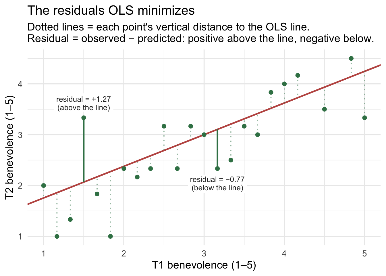
For a clean view, we plotted one representative participant per unique baseline score (23 participants in total — for a participant who answered all six items, the 6-item-average scale can take only 25 distinct values, and 23 of them appear in this sample). Notice that a handful of those participants sit very close to the line; others are well above or below. OLS doesn’t care that the line passes through any specific point — it cares that the whole bundle of squared residuals (across all 173 control participants) is as small as possible.
Computing the regression equation with lm()
In R, fitting an SLR is one line of code. The lm() function (“linear model”) takes a formula of the form outcome ~ predictor and a data frame:
ctrl_mod <- lm(t2_benevolence ~ t1_benevolence, data = control)
ctrl_mod
Call:
lm(formula = t2_benevolence ~ t1_benevolence, data = control)

Coefficients:
   (Intercept)  t1_benevolence
        1.1326          0.6227
The default print just shows the coefficients. For a tidy data frame with each coefficient’s standard error, t-statistic, p-value, and confidence interval, we use broom::tidy():
ctrl_mod |> tidy(conf.int = TRUE)What each column holds. Each row is one coefficient, named in term. The other columns describe it: estimate (the coefficient itself), std.error (its uncertainty), conf.low/conf.high (its interval), statistic (its observed t, \(t_\text{obs}\) — the coefficient divided by its SE), and p.value (its test). The Inference section later in this Part unpacks each one.
The estimated regression equation is therefore
\[\widehat{\text{T2 benevolence}}_i \;=\; 1.133 \;+\; 0.623 \cdot \text{T1 benevolence}_i\]
In words: the predicted T2 benevolence equals 1.133 plus 0.623 times T1 benevolence.
Reading the coefficients
- Intercept \(b_0\) = 1.133 (SE = 0.159). Predicted T2 benevolence for a control-arm participant whose T1 benevolence is 0. Since the 1–5 scale doesn’t include 0, the intercept is an extrapolation — meaningful for plotting the line but not for direct interpretation.
- Slope \(b_1\) = 0.623 (SE = 0.050, 95% CI [0.523, 0.722]). Comparing two Hong Kong control-arm participants whose T1 benevolence differs by one point, the model predicts that the one with the higher baseline will score 0.623 points higher at T2, on average. The Inference section later in this Part explains what the SE and the CI tell us.
Centering: when zero isn’t a useful baseline
The intercept of 1.133 is mathematically correct — it’s where the OLS line crosses the y-axis — but it’s hard to interpret. It tells us the predicted T2 benevolence for a participant whose baseline benevolence is 0, but nobody in the data has a baseline of 0. The 1–5 scale starts at 1, and the actual minimum baseline in our control sample is 1.00. So the intercept is forecasting something we’d never see — an extrapolation to a value off the edge of the scale.
This is a recurring problem in regression: zero is often not a meaningful value for the predictor(s). For T1 benevolence (1–5), zero is impossible; for age in years, zero is “newborn”; for income, zero is “no income,” which is meaningful only if the sample includes people near it. When zero is impossible or far outside the data, the intercept is technically correct but practically uninterpretable.
So what would a more useful intercept look like? One anchored to a meaningful value of baseline benevolence, for example the average baseline score rather than an impossible score of zero. Can we redefine the predictor so that \(x = 0\) represents that useful reference point?
We can. The fix is centering: subtract the mean of the predictor before fitting. The reparameterized predictor has the same shape and the same SD as the original — but its zero is now the sample mean of the predictor, which lies within the observed range and has a straightforward interpretation.
Building the centered predictor
In our control sample, the mean baseline benevolence is
control |> summarize(M_t1 = mean(t1_benevolence) |> round(3))Centering just means subtracting that number from every participant’s T1 score:
control_centered <- control |>
  mutate(t1_benevolence.c = t1_benevolence - mean(t1_benevolence))

control_centered |>
  summarize(
    M_centered = mean(t1_benevolence.c) |> round(3),
    SD_centered = sd(t1_benevolence.c)   |> round(3)
  )
The centered predictor has mean 0 by construction. Its SD is unchanged (centering shifts the mean but doesn’t squeeze or stretch the spread). Someone whose original T1 was the sample mean (3.05) now has a centered T1 of 0; someone whose original T1 was 4 has a centered T1 of 0.95; someone whose original T1 was 1 has a centered T1 of -2.05. The .c suffix is a useful naming convention — “centered version of t1_benevolence.”
Refitting with the centered predictor
ctrl_mod_c <- lm(t2_benevolence ~ t1_benevolence.c, data = control_centered)
ctrl_mod_c |> tidy(conf.int = TRUE)
Now compare the two fitted models. The regression line itself does not change: the slope, fitted values, residuals, and overall model fit are identical. What changes is the way that same line is parameterized around \(x = 0\), especially the intercept:
| Quantity | Uncentered (t1_benevolence) | Centered (t1_benevolence.c) | Notes |
|---|---|---|---|
| Intercept \(b_0\) | 1.133 | 3.029 | Different — and the centered version is interpretable |
| Intercept’s SE (so its t, CI, and p) | 0.159 | 0.044 | Different — it now describes the prediction at average \(x\) |
| Slope \(b_1\) | 0.623 | 0.623 | Identical |
| Slope’s SE (so its t, CI, and p) | 0.050 | 0.050 | Identical |
The fitted model hasn’t changed; its coordinate system has. Centering moves the predictor’s zero point from T1 = 0 to T1 = 3.05, the sample mean. Because of that shift, the intercept changes, and so do the intercept’s SE, t-statistic, confidence interval, and p-value. But the slope and its inference, the fitted values, the residuals, and the model’s overall fit (which the Model fit section below measures) are unchanged.
The new intercept now has a plain-language meaning: 3.029 is the predicted T2 benevolence for a control participant at average baseline benevolence. That’s exactly the kind of “anchor a typical person” interpretation we want from a regression intercept. And it is the simple control-arm mean of T2 (≈ 3.03; identical up to display rounding) — because the OLS line passes through the point (\(\bar{x}, \bar{y}\)), so the predicted T2 at the average T1 is exactly \(\bar{y}\).
Visualizing what centering does
The two fits draw the same line through the same data. All centering does is slide the y-axis along the predictor scale so that the line’s height at \(x = 0\) corresponds to “average baseline” instead of “baseline of 0”:
Show the code that built this figure
# The same line, two parameterizations: one slope, two intercepts
int_raw   <- ctrl_mod   |> coef() |> pluck("(Intercept)")
slope_raw <- ctrl_mod   |> coef() |> pluck("t1_benevolence")
int_cen   <- ctrl_mod_c |> coef() |> pluck("(Intercept)")
slope_cen <- ctrl_mod_c |> coef() |> pluck("t1_benevolence.c")

p_uncentered <- control |>
  ggplot(aes(x = t1_benevolence, y = t2_benevolence)) +
  geom_jitter(width = 0.05, height = 0.05, alpha = 0.30,
              color = "#3A8055", size = 1.4) +
  geom_abline(intercept = int_raw, slope = slope_raw,
              color = "#C05852", linewidth = 1.2) +
  geom_vline(xintercept = 0, color = "#1C2433",
             linetype = "dashed", linewidth = 0.5) +
  geom_point(aes(x = 0, y = int_raw), inherit.aes = FALSE,
             color = "#C05852", size = 4) +
  annotate("label", x = 0.5, y = int_raw + 0.4,
           label = sprintf("intercept = %.3f\n(extrapolation —\nT1 = 0 is off scale)", int_raw),
           color = "#C05852", fontface = "bold", fill = "white",
           label.size = 0, hjust = 0) +
  scale_x_continuous(breaks = 0:5) +
  scale_y_continuous(breaks = 0:5) +
  labs(
    x = "T1 benevolence (1–5)", y = "T2 benevolence (1–5)",
    title = "Uncentered: zero is off the 1–5 scale"
  )

p_centered <- control_centered |>
  ggplot(aes(x = t1_benevolence.c, y = t2_benevolence)) +
  geom_jitter(width = 0.05, height = 0.05, alpha = 0.30,
              color = "#3A8055", size = 1.4) +
  geom_abline(intercept = int_cen, slope = slope_cen,
              color = "#C05852", linewidth = 1.2) +
  geom_vline(xintercept = 0, color = "#1C2433",
             linetype = "dashed", linewidth = 0.5) +
  geom_point(aes(x = 0, y = int_cen), inherit.aes = FALSE,
             color = "#C05852", size = 4) +
  annotate("label", x = 0.3, y = int_cen + 0.4,
           label = sprintf("intercept = %.3f\n(predicted T2 at\naverage baseline)", int_cen),
           color = "#C05852", fontface = "bold", fill = "white",
           label.size = 0, hjust = 0) +
  scale_x_continuous(breaks = -3:2) +
  scale_y_continuous(breaks = 0:5) +
  labs(
    x = "T1 benevolence — centered (mean 0)", y = "T2 benevolence (1–5)",
    title = "Centered: zero is the average baseline"
  )

p_uncentered + p_centered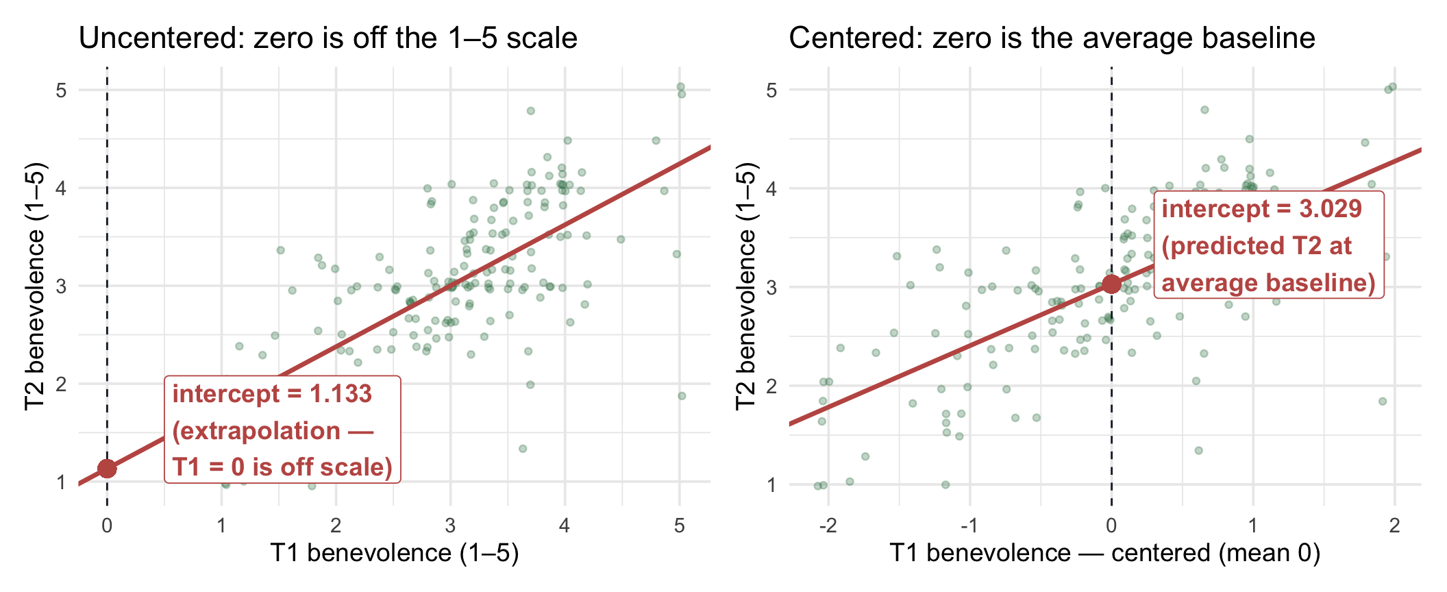
The two clouds are exactly the same shape, just slid horizontally by 3.05 units (the mean of T1). The OLS line is exactly the same line. What changes is the location of the y-axis and therefore the interpretation of where the line crosses it.
Centering — the key intuitions
- Centering does not change the fitted relationship. The slope, fitted values, residuals, overall model fit, and the slope’s inference are unchanged.
- The intercept’s own SE, CI, t, and p can change, because those quantities now refer to the predicted outcome at a different value of \(X\).
- Centering shifts the meaning of the intercept, from “predicted \(y\) when \(x = 0\)” to “predicted \(y\) at average \(x\)”. When zero isn’t a meaningful value (as for benevolence on a 1–5 scale, an IQ score, or age in an adult sample), centering gives the intercept a plain-language anchor.
- Centering doesn’t change the slope’s interpretation, only the intercept’s. The slope is still “the predicted difference in \(y\) between people one unit apart on \(x\)” — and two people one unit apart on centered \(x\) are one unit apart on uncentered \(x\) too.
- M11 will lean on centering, because in MLR the intercept’s interpretation gets compounded across multiple predictors. With several predictors, centering a continuous predictor makes zero correspond to that predictor’s mean. The intercept then represents the predicted outcome when each centered continuous predictor is at its mean and each categorical predictor is at its reference level.
Centering vs standardizing — same idea, different scaling. Centering subtracts the mean (so the new variable has mean 0). Standardizing (or z-scoring) subtracts the mean and divides by the SD (so the new variable has mean 0 and SD 1). Centering preserves the original units; standardizing makes the variable unit-free. We use centering again in M11; standardizing returns later in this Module (in the Correlation and standardized regression section), where standardizing both the predictor and the outcome makes the slope equal the correlation coefficient \(r\).
Predicted values and residuals — by hand
From here on, we return to the uncentered model, ctrl_mod, so predictions use raw T1 scores, which are easier to plug in. Because centering doesn’t change the line, the predictions, residuals, and fit would be the same with either version.
To make the equation concrete, let’s predict T2 benevolence for a hypothetical control-arm participant who scored T1 = 4 on the benevolence scale. Before you compute: 4 is above the average baseline, and the slope is less than 1, so will the prediction land above or below 4? (This is the regression-toward-the-mean tilt from earlier, about to show up in one person’s number.)
\[\widehat{y} \;=\; 1.133 \;+\; 0.623 \cdot 4 \;\approx\; 3.623\]
If their actual T2 benevolence happened to be 4.5, the residual would be
\[e \;=\; y - \widehat{y} \;=\; 4.5 - 3.623 \;\approx\; 0.877\]
A positive residual means the participant scored higher than the model predicted; a negative residual means lower.
broom::augment() adds predicted values and residuals as columns to the original data frame:
ctrl_mod |>
  augment() |>
  select(t1_benevolence, t2_benevolence, .fitted, .resid) |>
  slice_head(n = 8)
The .fitted column is \(\hat{y}_i\) for each participant; .resid is \(y_i - \hat{y}_i\). One arithmetic check: the residuals sum to zero (within numerical roundoff), a property of OLS. And one property you can’t see in the output: the SSE (the sum of squared residuals) is the smallest it can be over all possible lines.
ctrl_mod |>
  augment() |>
  summarize(
    sum_residuals = sum(.resid) |> round(6),
    SSE = sum(.resid^2) |> round(2)
  )
Model fit: R², \(\sigma\), and what “well-fit” means
Two summary statistics tell you how well the line fits the cloud. The first is R² — the proportion of the variation in \(Y\) that the predictor accounts for.
R² — proportion of variance explained
The total variation in T2 benevolence is the total sum of squares:
\[\text{SST} \;=\; \sum_i \left(y_i - \bar{y}\right)^2\]
Of that total, the predictor explains some part — the regression sum of squares:
\[\text{SSR} \;=\; \sum_i \left(\hat{y}_i - \bar{y}\right)^2\]
— and the rest is the error sum of squares (SSE — the sum of the squared residuals, which is what OLS minimized):
\[\text{SST} \;=\; \text{SSR} \;+\; \text{SSE}\]
You’ve seen this split before. M09’s one-way ANOVA divided the total variation, \(SS_\text{total}\), into \(SS_\text{between}\) (group means vs the grand mean) and \(SS_\text{within}\) (each score vs its own group’s mean). Regression makes the same split. The only change is what supplies each person’s prediction: in ANOVA it was their group’s mean; here it is the line’s \(\hat{y}_i\). So SST plays the role of \(SS_\text{total}\), SSR the role of \(SS_\text{between}\), and SSE the role of \(SS_\text{within}\). In Part 3, with site as the predictor, you’ll see a regression and M09’s one-way ANOVA give identical results.
These familiar OLS identities assume an intercept. Throughout PSY 652, our regression models include an intercept, which is R’s default. Under that setup, residuals sum to zero, the fitted line passes through \((\bar{x}, \bar{y})\), \(\text{SST} = \text{SSR} + \text{SSE}\), and, with one continuous predictor, \(R^2 = r^2\). Models fit without an intercept behave differently.
R² is the regression-share of the total:
\[R^2 \;=\; \frac{\text{SSR}}{\text{SST}} \;=\; 1 - \frac{\text{SSE}}{\text{SST}}\]
broom::glance() reports it directly:
ctrl_mod |> glance()For our control-arm regression, R² = .473 — meaning baseline benevolence accounts for about 47% of the variation in 2-week follow-up benevolence within the control arm. The remaining 53% is variation the predictor doesn’t capture: idiosyncratic life events between the two timepoints, measurement noise, the participant’s mood on the day of the second survey, and so on.
How large is an R²?
There is no universal cutoff for a “small,” “medium,” or “large” R². Its practical meaning depends on the outcome, the research setting, the reliability of the measures, and what kinds of predictors are realistically available. (You may see .01, .09, and .25 quoted as Cohen’s benchmarks for R². Those are his benchmarks for a correlation, .10, .30, and .50, squared; they aren’t his regression benchmarks.)
Here, R² = .473 is substantial: baseline benevolence accounts for about 47% of the observed variation in the same construct measured two weeks later, which makes sense for a repeated measure of the same psychological construct. The useful question is therefore not simply “Is this R² large?” but “How much variation does this model account for, and is that amount useful in this research context?”
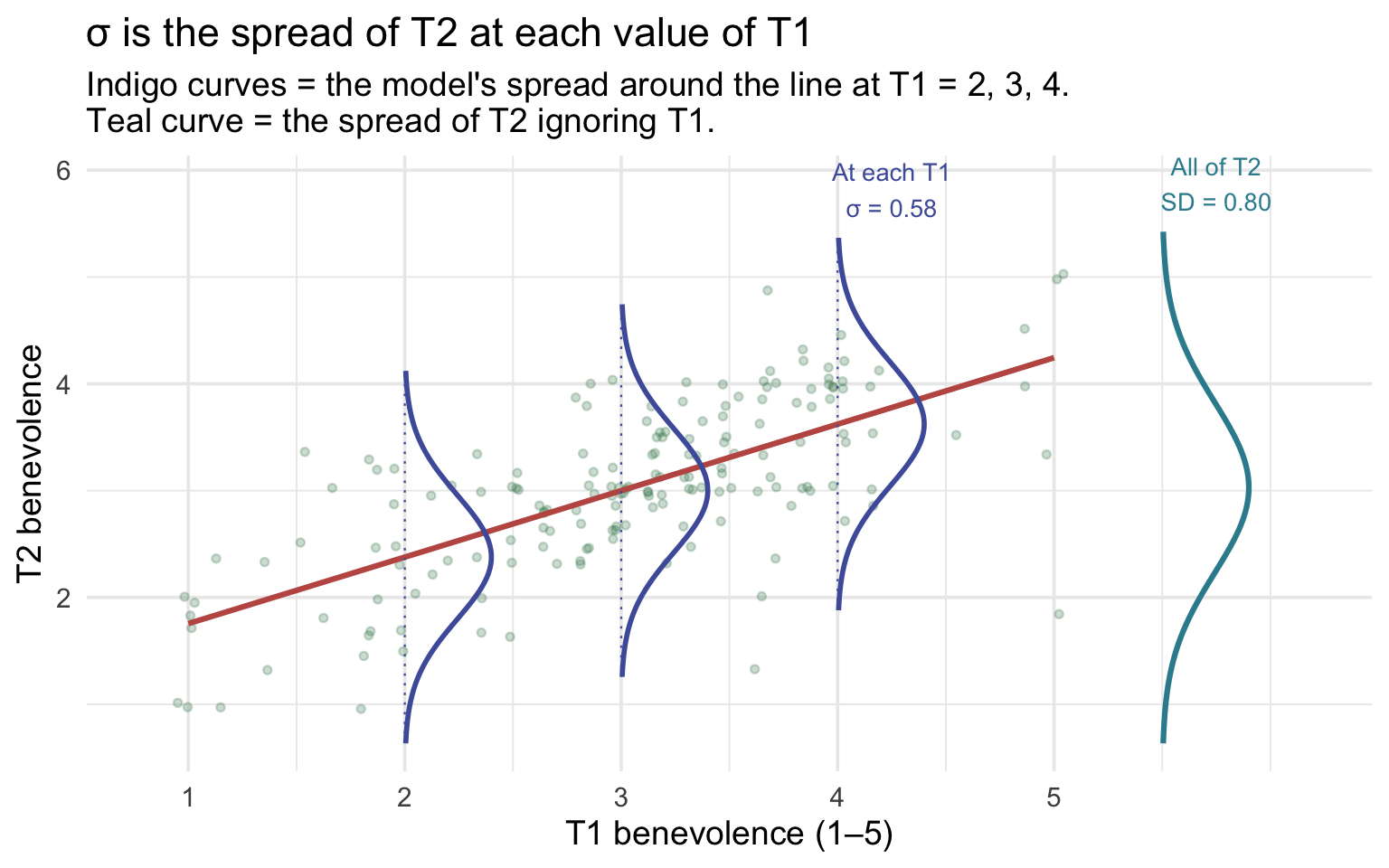
\(\sigma\) — the residual standard error
The second fit summary is \(\sigma\) — the residual standard error (closely related to the root mean square error). It’s the model’s estimate of the SD of the population errors — the typical scale of the vertical scatter around the regression line, in the units of \(Y\) — computed from the residuals with an \(n - 2\) degrees-of-freedom correction (so it’s not simply sd() of the residuals).
\[\sigma \;=\; \sqrt{\frac{\text{SSE}}{n - 2}}\]
The denominator is \(n - 2\) rather than \(n\) because the line uses up two degrees of freedom (one for \(b_0\), one for \(b_1\)); the formula is the regression analog of the SD’s \(n - 1\) denominator. From glance(), \(\sigma\) = 0.581 for our model. So prediction errors around the fitted line commonly vary on the scale of roughly 0.58 of a benevolence point.
Compare that to \(SD_y\) = 0.798: if we had no predictor and just predicted T2 benevolence as the overall mean, our typical error would be \(SD_y\) ≈ 0.80. With T1 benevolence as a predictor, the typical error drops to \(\sigma\) ≈ 0.581. The drop from \(SD_y\) to \(\sigma\) tells a story closely related to R²: once T1 is used to predict T2, the remaining scatter around the predictions is smaller than the original spread of T2 around its mean.
\(\sigma\) is the spread at each value of \(X\). Take everyone with the same baseline score, say T1 = 3. They don’t all land on the same T2 score; they scatter above and below the line’s prediction for that baseline. The regression model describes that scatter as roughly Normal, centered on \(\hat{y}\), with standard deviation \(\sigma\), and it assumes the same \(\sigma\) at every value of T1. That is a conditional spread: the spread of T2 among people who share a T1 score. \(SD_y\) is the marginal spread: the spread of T2 when we ignore T1 entirely. Knowing someone’s baseline narrows the range of plausible follow-up scores, and the gap between the two spreads is how much the predictor reduces our uncertainty about T2.
A concrete reading of \(\sigma\). If the model’s errors really are Normal with SD \(\sigma\), then among people who share a T1 score, about two-thirds would land within ±\(\sigma\) (± 0.58 points) of the line’s prediction, and about 95% within ±2\(\sigma\) (± 1.16 points). That’s a property of the Normal-error model, not a guarantee about any particular sample, but it gives \(\sigma\) a scale you can picture. It’s also the person-to-person spread that the prediction interval, later in this Part, is built from.
Show the code that built this figure
sd_y      <- control |> pull(t2_benevolence) |> sd()
m_y       <- control |> pull(t2_benevolence) |> mean()
fit_b0    <- ctrl_mod |> coef() |> pluck("(Intercept)")
fit_b1    <- ctrl_mod |> coef() |> pluck("t1_benevolence")
fit_sigma <- ctrl_mod |> glance() |> pull(sigma)

# A sideways Normal curve: heights become horizontal offsets from x0
side_bell <- function(x0, center, spread, width = 0.4) {
  tibble(y = seq(center - 3 * spread, center + 3 * spread, length.out = 200)) |>
    mutate(x = x0 + width * dnorm(y, center, spread) / dnorm(0, 0, spread),
           x0 = x0)
}

conditional_bells <- map_dfr(c(2, 3, 4), \(x0) side_bell(x0, fit_b0 + fit_b1 * x0, fit_sigma))
marginal_bell     <- side_bell(5.5, m_y, sd_y)

ggplot() +
  geom_jitter(data = control, aes(x = t1_benevolence, y = t2_benevolence),
              width = 0.05, height = 0.05, alpha = 0.25, color = "#3A8055", size = 1.2) +
  # the fitted line over the observed T1 range only, so it doesn't run into the teal curve
  annotate("segment", x = 1, xend = 5, y = fit_b0 + fit_b1 * 1, yend = fit_b0 + fit_b1 * 5,
           color = "#C05852", linewidth = 1.1) +
  geom_segment(data = tibble(x0 = c(2, 3, 4)),
               aes(x = x0, xend = x0, y = fit_b0 + fit_b1 * x0 - 3 * fit_sigma,
                   yend = fit_b0 + fit_b1 * x0 + 3 * fit_sigma),
               color = "#4E5EAA", linewidth = 0.4, linetype = "dotted") +
  geom_path(data = conditional_bells, aes(x = x, y = y, group = x0),
            color = "#4E5EAA", linewidth = 1) +
  geom_path(data = marginal_bell, aes(x = x, y = y), color = "#348C9E", linewidth = 1.1) +
  annotate("text", x = 5.75, y = m_y + 3 * sd_y + 0.45, color = "#348C9E", size = 3.6,
           label = sprintf("All of T2\nSD = %.2f", sd_y)) +
  annotate("text", x = 4.25, y = fit_b0 + fit_b1 * 4 + 3 * fit_sigma + 0.45, color = "#4E5EAA",
           size = 3.6, label = sprintf("At each T1\nσ = %.2f", fit_sigma)) +
  scale_x_continuous(breaks = 1:5) +
  coord_cartesian(xlim = c(0.8, 6.2)) +
  labs(
    x = "T1 benevolence (1–5)", y = "T2 benevolence",
    title = "σ is the spread of T2 at each value of T1",
    subtitle = "Indigo curves = the model's spread around the line at T1 = 2, 3, 4.\nTeal curve = the spread of T2 ignoring T1."
  )
How \(\sigma\) and R² connect. Because R² is the share of the outcome’s variance the line accounts for, the variance left over is about \((1 - R^2)\) times the original. Take square roots, and
\[\sigma \;\approx\; SD_y \sqrt{1 - R^2} \;=\; 0.798 \times \sqrt{1 - .473} \;\approx\; 0.580\]
which lands within a rounding error of the actual \(\sigma\) = 0.581. The relationship is approximate only because \(SD_y\) divides by \(n - 1\) while \(\sigma\) divides by \(n - 2\); with 173 participants, that difference barely shows. The practical reading: as R² rises, \(\sigma\) falls. A model that accounts for more of the variation leaves less scatter around its line.
Inference: where the standard errors and CIs come from
Up to this point we’ve treated the regression line as a description of our control sample — point estimates of intercept and slope, plus measures of how well the line fits. But every inferential step you took in M07–M09 was about generalizing from a sample to a population. The same logic applies here. Our 173-person control sample is one possible draw from a much larger population, and the slope of 0.623 we computed is one possible estimate of the unknown population slope. A different control sample of the same size would have produced a slightly different slope — and we want to know how big that “slightly” is. This population interpretation assumes it’s reasonable to treat these participants as draws from a target population. Random assignment to treatment doesn’t by itself make the study sample representative of any population; that depends on how participants were recruited, the sampling ideas from M05.
This subsection unpacks where the tidy() output’s standard error, t-statistic, p-value, and 95% CI columns come from, and how to read them. Then it introduces a second flavor of inference that’s specific to regression: prediction intervals for individual cases vs confidence intervals for the line itself.
This is the longest stretch in the Module — here’s the map
We’ll pin down the slope’s uncertainty two ways — by bootstrap (simulation) and by the closed-form formula R actually uses — compare what they say, then build the slope’s confidence interval from that SE, and then meet the hypothesis test and the F-test, two equivalent ways to test the slope. Then we’ll separate a CI for the line from a PI for an individual. If you’re skimming on a first pass, carry away just this: the slope has a standard error, and that SE is what the CI, the t-statistic, and the p-value are all built from. Everything else is showing you why that SE is trustworthy.
Parameters vs estimates: a notational convention
When we talk about a regression model abstractly, we distinguish two versions of the same equation. The population equation uses Greek letters for the true, unknown parameters that govern the population:
\[\underbrace{Y_i}_{\text{observed outcome}} \;=\; \underbrace{\beta_0 \;+\; \beta_1 X_i}_{\text{true line in the population}} \;+\; \underbrace{\epsilon_i}_{\text{true error, averaging 0 at every } X}\]
- \(\beta_0\) — the true population intercept.
- \(\beta_1\) — the true population slope.
- \(\sigma_\epsilon\) — the true population residual SD (the standard deviation of the error term). One notational detail to accept: by the Greek-vs-Latin rule below, the estimate ought to wear a hat or a Latin letter — some books write \(\hat{\sigma}\) or \(s_e\) — but R’s glance() names its estimate column
sigma, and this Module follows R’s naming. When you see unadorned \(\sigma\) in output or prose here, it is the sample estimate of \(\sigma_\epsilon\). - \(\epsilon_i\) — the true random error for person \(i\) in the population. For the OLS slope to be unbiased, the key condition is that the error has mean zero conditional on \(X\): \(E(\epsilon_i \mid X_i) = 0\). That “conditional on \(X\)” matters — the error can average to zero overall while still being systematically related to the predictor, and then the slope can be biased. For the usual small-sample t-tests and CIs, the classical model additionally assumes the errors are independent, of constant variance, and approximately Normal; the Normality part matters mainly for exact small-sample p-values and CIs for the coefficients. It matters more directly when you predict individuals: a prediction interval leans on the shape of the error distribution at any sample size, as the prediction-interval section below explains. (Module 12 takes up all of these diagnostics.)
A preview of what M12 will check
Right now we’re learning to fit and interpret regression models. Before trusting their inference, though, we will eventually ask several separate questions:
- Is the mean relationship adequately modeled as linear?
- Are the observations sufficiently independent?
- Is the residual variance reasonably constant across the predictor?
- Are the error-distribution assumptions good enough for the inferential method we’re using? (Approximately Normal errors give exact small-sample t and F inference, and they matter at any sample size for prediction intervals for individuals.)
We’ll also inspect influential observations: not because “having no influential points” is a formal model assumption, but because a small number of observations can sometimes exert disproportionate control over the fitted coefficients.
M12 turns each of these into a diagnostic workflow. For now, the important point is simply that “the scatter looks roughly straight” is only one part of checking a regression model.
The sample equation uses Latin letters for our sample-based estimates of those population parameters:
\[\underbrace{\hat{y}_i}_{\text{predicted from our sample}} \;=\; \underbrace{b_0 \;+\; b_1 x_i}_{\text{OLS line fit to our sample}} \qquad\qquad e_i \;=\; y_i - \hat{y}_i\]
- \(b_0\) — our estimate of \(\beta_0\) from this sample.
- \(b_1\) — our estimate of \(\beta_1\) from this sample.
- \(e_i\) — the observed residual for person \(i\) — what’s left after this sample’s line predicts \(y_i\).
Greek = the truth; Latin = our best guess from one sample. The goal of inference is to use what we know (Latin) to say something quantified about what we don’t (Greek). For our control regression: \(b_1 = 0.623\) is our best guess for the unknown \(\beta_1\); the rest of this section is about how precise that guess is.
The bootstrap view of sample-to-sample variability
In M07 we built intuition for sampling variability by bootstrap resampling — drawing many resamples from our data and seeing how the statistic of interest varies across them. The same idea applies to a regression. If we resample our 173 control participants with replacement and re-fit the regression on each resample, we get a new line each time — a new intercept and a new slope. The spread of those many lines tells us how much our regression would wobble across different samples drawn from the same population.
The question driving this whole stretch: if we’d happened to catch a different 173 Hong Kong controls, how different a line would we have drawn? The bootstrap answers it by construction — redraw, refit, repeat — and the spread of the lines you get estimates the slope’s uncertainty.
Step 1: Look at nine bootstrap resamples
Let’s start by drawing nine resamples and fitting our regression on each. Each panel below is one bootstrap resample (a random draw of 173 rows from the control arm, with replacement); the colored line is that resample’s OLS fit. Before you read on, compare two panels directly — put panel 4’s line next to panel 7’s. Same procedure, same source data, visibly different tilt: that wobble is what we’re about to measure.
ctrl_n <- nrow(control)   # the sample size; each resample matches it

set.seed(652)
boot9 <- map_dfr(1:9, function(i) {
  control |> slice_sample(n = ctrl_n, replace = TRUE) |>
    mutate(resample = i)
})

panel_colors <- c("#348C9E", "#C05852", "#AD872B", "#4E5EAA", "#945297",
                  "#3A8055", "#7C9CBF", "#D88D3D", "#5E8A6F")

boot9 |>
  ggplot(aes(x = t1_benevolence, y = t2_benevolence,
             color = factor(resample))) +
  geom_jitter(width = 0.05, height = 0.05, alpha = 0.10, size = 0.7) +
  geom_smooth(method = "lm", formula = y ~ x, se = FALSE,
              linewidth = 1.0) +
  scale_color_manual(values = panel_colors, guide = "none") +
  facet_wrap(~ paste("Resample", resample), ncol = 3) +
  scale_x_continuous(breaks = 1:5) +
  scale_y_continuous(breaks = 1:5) +
  labs(
    x = "T1 benevolence (1–5)", y = "T2 benevolence (1–5)",
    title = "Nine bootstrap resamples — nine slightly different lines"
  )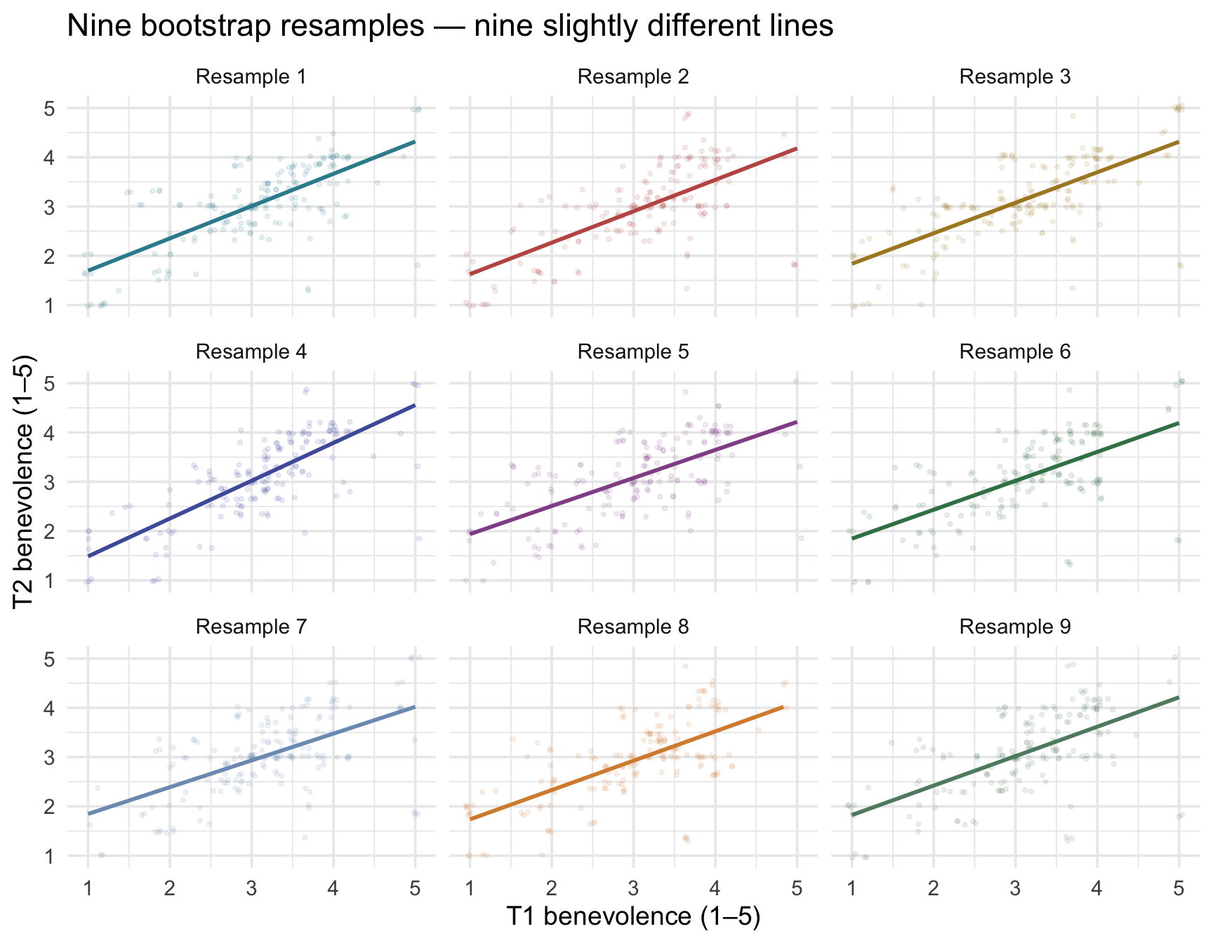
Each panel’s line passes through that resample’s cloud, and the lines are clearly similar but not identical. Each carries its own intercept and slope, summarized in the table below:
Show the code that built this table
set.seed(652)
boot9_summary <- map_dfr(1:9, function(i) {
  bs <- control |> slice_sample(n = ctrl_n, replace = TRUE)
  m  <- lm(t2_benevolence ~ t1_benevolence, data = bs)
  g  <- m |> glance()
  tibble(
    resample = i,
    intercept = m |> coef() |> pluck("(Intercept)") |> round(3),
    slope = m |> coef() |> pluck("t1_benevolence") |> round(3),
    R_sq = g |> pull(r.squared) |> round(3),
    sigma = g |> pull(sigma) |> round(3)
  )
})

boot9_summary
The intercepts cluster around 1.141 and the slopes cluster around 0.619 — but each resample gives a slightly different pair. Same data-generating process, different specific draws.
Step 2: Stack 1,000 bootstrap lines on a single chart
Nine resamples give a hint of the variability; 1,000 makes the pattern visually unmistakable. In the figure below each gray line is one resample’s OLS fit and the rose line is the fit to the original sample. We re-fit the regression on each of 1,000 bootstrap resamples and plot all 1,000 lines on top of each other:
set.seed(652)
boot1000 <- map_dfr(1:1000, function(i) {
  bs <- control |> slice_sample(n = ctrl_n, replace = TRUE)
  m  <- lm(t2_benevolence ~ t1_benevolence, data = bs)
  tibble(rep = i,
         intercept = m |> coef() |> pluck("(Intercept)"),
         slope = m |> coef() |> pluck("t1_benevolence"))
})

ggplot() +
  geom_jitter(data = control,
              aes(x = t1_benevolence, y = t2_benevolence),
              width = 0.05, height = 0.05, alpha = 0.30,
              color = "#3A8055", size = 0.8) +
  geom_abline(data = boot1000,
              aes(intercept = intercept, slope = slope),
              color = "#8C929C", alpha = 0.10, linewidth = 0.4) +
  geom_abline(intercept = ctrl_mod |> coef() |> pluck("(Intercept)"),
              slope = ctrl_mod |> coef() |> pluck("t1_benevolence"),
              color = "#C05852", linewidth = 1.6) +
  scale_x_continuous(breaks = 1:5) +
  scale_y_continuous(breaks = 1:5) +
  labs(
    x = "T1 benevolence (1–5)",
    y = "T2 benevolence (1–5)",
    title = "1,000 bootstrap regression lines",
    subtitle = "Each gray line is one resample's OLS fit. The rose line is the original-sample fit.\nThe cloud of gray lines is what a 95% CI for the regression line is trying to summarize."
  )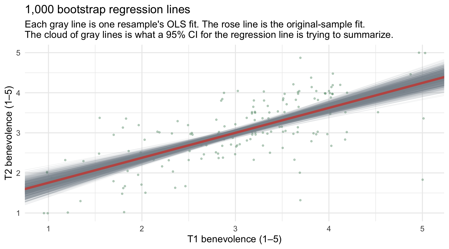
Two things to notice — both substantively important:
- The lines all pass near the data’s centroid. The centroid is the point \((\bar{x}, \bar{y})\): the average T1 paired with the average T2. An OLS line with an intercept always passes exactly through its own data’s centroid. Each resample has a slightly different centroid, but all of them sit close to the original one, so no matter which 173 participants you draw, the line is anchored near the average T1 and the average T2. That’s why the gray lines pinch tightest near \(\bar{x}\) ≈ 3.05.
- The lines fan out at the extremes. At T1 = 1 (the bottom of the scale) and T1 = 5 (the top), the gray cloud is visibly thicker. That’s because at extreme values of \(X\), even a small wobble in the slope translates into a large wobble in the predicted \(\hat{y}\).
This fanning pattern visualizes the uncertainty that a regression-line confidence band summarizes. The band answers one question: at each value of T1, where could the population line plausibly run? Pick any T1 value and look straight up the plot: the gray lines cross that spot over a range of heights. That range is our uncertainty about the average T2 for people with that baseline. Take the middle 95% of those heights at each T1 value (the 2.5th and 97.5th percentiles of the 1,000 bootstrap predictions there), line them up across every T1 value, and you get a pointwise bootstrap 95% confidence band, narrow near the middle of the data and wider at the edges. The band describes the line (an average), not individual people, who scatter much more widely, as the section on prediction intervals will show. The parametric 95% CI for the line — plotted as a rose ribbon in the CI for the line vs PI for individuals section below — is the same hourglass shape, computed by formula instead of by simulation. They’re two ways of estimating the same quantity — and the next step shows that the two routes don’t agree exactly for the slope’s SE.
Step 3: Extract the standard error and CI
A thousand plausible slopes is a picture; a report needs numbers. How do you compress the whole cloud into an SE and a 95% CI? Exactly the way M07 taught you: take the SD and percentiles of the 1,000 bootstrap slopes:
boot1000 |>
  summarize(
    boot_se = sd(slope),
    boot_ci_lo = quantile(slope, 0.025),
    boot_ci_hi = quantile(slope, 0.975)
  )
Two things to take away. First: the SD of bootstrap slopes (≈ 0.0621) and the parametric SE that tidy() reports (0.0503) are estimates of the same quantity by different routes — and they are close, though look closely: the bootstrap comes out noticeably larger here. Second, the same pattern in interval form: the bootstrap 95% percentile CI for the slope is [0.502, 0.741], somewhat wider than the parametric [0.523, 0.722], though both tell the same substantive story — the slope sits far from 0 and below 1. That gap is not Monte Carlo error, the small random wobble that comes from estimating by simulation (you met the term in the M08 pre-study), because it persists across seeds. The two methods rely on different approximations and assumptions, so they need not agree exactly. One potentially relevant feature of these data is that the residual spread is not perfectly constant across \(X\), a pattern we’ll learn to diagnose explicitly in M12. The formula-based SE assumes the scatter around the line is the same at every value of \(X\); resampling whole participants doesn’t make that assumption, so when the scatter varies, the two estimates can drift apart. For now, the important result is that both approaches tell the same substantive story about the slope.
The same bootstrap with M07’s rep_slice_sample()
The slice_sample() loop above shows every moving part, which is why this Module teaches it. The resampling tool you used in M07 and the M09 lab, rep_slice_sample(), does the same job in fewer lines: draw all 1,000 resamples at once, keep them apart with group_by(replicate), and refit the line inside each one. One argument you may remember from the M09 lab: prop = 1 sets each resample’s size as a proportion of the data, and 1 means 100%, so every resample has as many rows as control. It does the same job as n = ctrl_n in the loop above, without your having to look up the sample size; a bootstrap needs each resample to be the same size as the original sample. A smaller resample would make the estimates wobble more than a real sample of this size does, and the SE would come out too large.
set.seed(652)
boot_slopes <- control |>
  rep_slice_sample(prop = 1, replace = TRUE, reps = 1000) |>
  group_by(replicate) |>
  summarize(slope = lm(t2_benevolence ~ t1_benevolence) |> coef() |> pluck("t1_benevolence"))

boot_slopes |>
  summarize(
    boot_se    = sd(slope),
    boot_ci_lo = quantile(slope, 0.025),
    boot_ci_hi = quantile(slope, 0.975)
  )
Read the pipeline one step at a time:
- rep_slice_sample(prop = 1, replace = TRUE, reps = 1000) draws 1,000 resamples, each the same size as control and drawn with replacement, and labels them with a
replicatecolumn running from 1 to 1,000. - group_by(replicate) keeps the resamples apart, so the next step runs once per resample.
- Inside summarize(), lm() refits the line using only the current resample’s rows; coef() returns that fit’s two coefficients; and pluck("t1_benevolence") keeps the slope. pluck() comes from the purrr package, part of the tidyverse, and pulls one named element out of a vector;
pluck("(Intercept)")would keep the intercept instead. - The result has one row per resample, with its slope in the column you named slope. The second pipeline turns those 1,000 slopes into a bootstrap SE and a 95% percentile CI.
The two approaches produce the same kind of bootstrap distribution. The pre-study’s bootstrap activities use this shorter form, so you’ll run it yourself there.
The parametric route — why we don’t have to bootstrap every time
The conventional OLS standard-error formula assumes independent observations and constant error variance. Normal errors give the familiar t and F reference distributions exactly in small samples; with larger samples, coefficient inference can often tolerate substantial departures from Normality. Large \(n\), however, does not by itself fix dependence or unequal error variance. Under those assumptions, the SE of the slope has a closed-form formula:
\[SE(b_1) \;=\; \frac{\sigma}{\sqrt{\sum_i (x_i - \bar{x})^2}} \;=\; \frac{0.581}{\sqrt{133.73}} \;\approx\; 0.0503\]
That is exactly the std.error that tidy() reports for the slope.
A smaller residual SD (the numerator) shrinks the SE — better-fit lines have more precise slopes. A wider spread of \(X\) (the denominator) shrinks it too — the wider the range of \(X\), the more information the data carry about the slope, and the more precisely \(b_1\) is identified. A regression with a tiny X-range is fundamentally less precise than one with a wide X-range, even at the same \(n\) and the same residual SD.
TipGoing further — the intercept’s standard error
The intercept’s SE has a similar formula, with one extra term:
\[SE(b_0) \;=\; \sigma\sqrt{\frac{1}{n} \;+\; \frac{\bar{x}^2}{\sum_i (x_i - \bar{x})^2}} \;=\; 0.581\sqrt{\frac{1}{173} \;+\; \frac{3.045^2}{133.73}} \;\approx\; 0.1593\]
again matching tidy(). The extra term, \(\bar{x}^2 / \sum_i (x_i - \bar{x})^2\), grows the further the mean of \(X\) sits from zero. Here \(\bar{x}\) ≈ 3.05, far from zero, so the intercept (a prediction at T1 = 0, outside the data) comes with a large SE. Center the predictor and \(\bar{x} = 0\): the extra term drops out, leaving \(SE(b_0) = \sigma / \sqrt{n}\) ≈ 0.0442. That is the smaller intercept SE in the Centering section’s table above.
The good news: you don’t actually have to compute these formulas by hand — R does it for you:
ctrl_mod |> tidy(conf.int = TRUE)The std.error column is what the formulas above evaluate to. For our slope: SE = 0.0503 — the closed-form counterpart of the bootstrap SD of 0.0621 you just simulated (and, as noted above, noticeably smaller here). The conventional formula and the bootstrap estimate the same underlying sampling uncertainty by different routes. The conventional SE uses the assumptions of the classical linear model; the pairs bootstrap approximates sampling variability by repeatedly resampling the observed \((X, Y)\) pairs. Neither approach is assumption-free, and disagreement between them can be a useful signal that the data deserve a closer look.
95% CI on the slope
Now we have the two numbers everything else is built from: the estimate and its standard error. The interval comes first, built exactly as M07 built every interval — step out some number of standard errors on either side of the estimate:
\[b_1 \;\pm\; t^*_{n-2, \, .025} \cdot SE(b_1) \;=\; 0.623 \;\pm\; 1.974 \cdot 0.0503 \;=\; [0.523, 0.722]\]
The multiplier \(t^*_{171, \, .025}\) ≈ 1.974 is the two-sided critical value at \(\alpha = .05\), which R reads off a t-distribution with \(n - 2\) degrees of freedom — qt(p = 0.975, df = 171), the same call M07 used for a mean. That is the whole computation: an estimate, its SE, and a multiplier that depends only on the confidence level and the df. The conf.low and conf.high columns of tidy(conf.int = TRUE) land at 0.523 and 0.722 — close to the bootstrap percentile CI of [0.502, 0.741], with the modest bootstrap-runs-wider gap discussed above.
Plain-language interpretation (read this carefully — it’s exactly the same long-run-procedure framing from M07): if we drew many control samples of n = 173 from the same population and built a 95% CI from each, about 95% of those intervals would contain the true population slope \(\beta_1\). The 95% lives in the procedure, not in this one interval. Our specific interval, [0.523, 0.722], either contains \(\beta_1\) or it doesn’t — we never get to know which. What’s useful here is the exclusion pattern. The interval excludes 0, so the data provide strong evidence of a positive population linear association between T1 and T2 benevolence. It also excludes a raw slope of 1. Because the two occasions use the same scale, that is consistent here with the standardized regression-toward-the-mean pattern discussed earlier; remember, though, that the correlation, not the raw slope by itself, is the cleanest scale-free measure of that shrinkage.
Hypothesis test on the slope
The statistic column above is \(t_\text{obs}\) for the slope — the observed t-statistic, defined exactly as M09’s parametric tests defined it:
\[t_\text{obs} \;=\; \frac{b_1 - \beta_1^{\text{null}}}{SE(b_1)} \;=\; \frac{0.623 - 0}{0.0503} \;\approx\; 12.4\]
The null value \(\beta_1^{\text{null}} = 0\) is the standard “no linear association” hypothesis: \(H_0: \beta_1 = 0\). In the population model, a zero slope means a flat line: the average T2 would be the same at every T1 score. Under \(H_0\), the t-statistic follows a t-distribution with \(df = n - 2\) degrees of freedom (one df used for the intercept, one for the slope). For our 173-person control sample, \(df = 171\).
The p.value column is the two-sided tail probability of seeing a t as far from zero as our \(t_\text{obs}\), under that null distribution. For our slope, p < .001 — vanishingly small. We reject \(H_0\): the data provide strong evidence that the population slope is not zero. For a test–retest slope, that conclusion is not surprising. A slope of 0 would mean that a person’s benevolence today tells us nothing about their benevolence two weeks later, which was never a serious possibility. Gelman, Hill, and Vehtari caution against leaning on tests of null hypotheses “that we know ahead of time cannot be true.” Here the more informative results are the slope’s size and its CI, which the previous section reported — including the fact that the CI excludes 1.
This is the M09 framework, applied to a regression coefficient. An observed statistic (\(t_\text{obs}\)), a reference distribution, the same critical value \(t^*\) = 1.974 the interval just used, a p-value — the main new ingredient is the formula for the SE. Notice that the test needed nothing the interval didn’t: the same estimate, the same SE, the same t-distribution on \(n - 2\) degrees of freedom.
The F-test: same hypothesis, told as a variance-explained vs variance-unexplained ratio
There’s a second, equivalent way to test \(H_0: \beta_1 = 0\) that’s important to recognize because it generalizes to multi-predictor regression (M11) and to ANOVA (M09 Test 2) — and because many published regression reports show it. The F-test asks the same null-hypothesis question, whether the population linear signal is zero, but frames the evidence as a ratio of model variation to residual variation rather than as a standardized coefficient.
To get there, we first split the outcome’s total variation into its two parts (three sums of squares in all).
The three sums of squares
Define the grand mean \(\bar{y}\) — what we’d predict for everyone if we had no predictor at all. Then for each participant, three quantities relate observed \(y_i\), predicted \(\hat{y}_i\), and the grand mean:
| Sum of squares | Formula | What it measures |
|---|---|---|
| Total (\(\text{SST}\)) | \(\sum_i (y_i - \bar{y})^2\) | Total variation in \(Y\) — what we’d be left to explain if the predictor were useless |
| Regression (\(\text{SSR}\)) | \(\sum_i (\hat{y}_i - \bar{y})^2\) | The part the line captures — how much each predicted value differs from the grand mean |
| Error (\(\text{SSE}\)) | \(\sum_i (y_i - \hat{y}_i)^2\) | The part the line misses — the SSE we minimized when fitting OLS |
These three quantities are linked by an identity:
\[\text{SST} \;=\; \text{SSR} \;+\; \text{SSE}\]
That is — every unit of variation in \(Y\) is either explained by the predictor (the regression part) or unexplained (the error part). There’s no third bucket.
ss_table <- control |>
  mutate(
    .fitted = predict(ctrl_mod),
    grand_mean = mean(t2_benevolence)
  ) |>
  summarize(
    SST = sum((t2_benevolence - grand_mean)^2),
    SSR = sum((.fitted - grand_mean)^2),
    SSE = sum((t2_benevolence - .fitted)^2)
  ) |>
  mutate(check = SSR + SSE)

ss_table |> mutate(across(everything(), \(x) round(x, 2)))
The check column is SSR + SSE — and matches SST exactly, confirming the identity.
Notice also that \(\text{SSR} / \text{SST}\) is exactly R²:
\[R^2 \;=\; \frac{\text{SSR}}{\text{SST}} \;=\; \frac{51.85}{109.63} \;\approx\; .473\]
— the same .473 that glance() reported above. That’s where R² comes from: the SS-decomposition view of “what fraction of variance the line explained.”
Degrees of freedom and mean squares
The next ingredient: degrees of freedom. Each sum of squares is divided by its df to produce a mean square (an average sum-of-squares-per-unit-of-information), the same step M09 took to turn \(SS_\text{between}\) and \(SS_\text{within}\) into \(MS_\text{between}\) and \(MS_\text{within}\):
- \(df_\text{regression} = 1\) — we used one parameter (the slope) to compute the regression-explained piece.
- \(df_\text{error} = n - 2 = 171\) — the df left after using two for the intercept and slope.
The two mean squares are
\[MSR \;=\; \frac{\text{SSR}}{df_\text{regression}} \;=\; \frac{51.85}{1} \;=\; 51.85\]
\[MSE \;=\; \frac{\text{SSE}}{df_\text{error}} \;=\; \frac{57.78}{171} \;\approx\; 0.338\]
You’ve actually already met MSE: it’s \(\sigma^2\) — the squared residual standard error from the Model fit section. The “typical squared miss” of the line. From glance(), \(\sigma\) ≈ 0.581, so \(\sigma^2 \approx\) 0.338. Same number.
The F-statistic
The F-statistic is the ratio of those two mean squares — the explained sum of squares per df vs the unexplained sum of squares per df:
\[F_\text{obs} \;=\; \frac{MSR}{MSE} \;=\; \frac{51.85}{0.338} \;\approx\; 153.5\]
For our model, \(F_\text{obs}\) = 153.5, which glance() reports as statistic:
ctrl_mod |> glance() |>
  select(r.squared, statistic, p.value, df, df.residual, sigma)
Read it as: “the regression mean square (the sum of squares the line accounts for, per regression df) is about 153 times the residual mean square (the leftover sum of squares, per residual df).” In short, the model’s signal per df is about 153 times the residual noise per df. Under \(H_0: \beta_1 = 0\), the F-statistic follows an F-distribution with \((df_\text{regression}, df_\text{error}) = (1, 171)\). A value of 153.5 sits far out in the right tail; the corresponding p-value is < .001 — same conclusion as the t-test.
\(t_\text{obs}^2 = F_\text{obs}\) (for SLR)
For a single-predictor regression, the F-test on the model and the t-test on the slope are exactly the same test, expressed in two notations. Specifically:
\[F_\text{obs} \;=\; t_\text{obs}^2\]
Verify with our numbers:
\[t_\text{obs}^2 \;=\; (12.39)^2 \;\approx\; 153.5 \;=\; F_\text{obs}\]
The p-values are identical too (both < .001). \(F_\text{obs}\) is \(t_\text{obs}\), squared. In SLR, you’d usually report just one — you’d pick the one that matches your reporting convention. And carry the practical corollary with you: whenever an F-test has one numerator df, its \(F_\text{obs}\) and the \(t_\text{obs}\) on the same comparison are the same result — take the square root before concluding that two analyses disagree. Most psychology papers report the t on the slope; some textbooks (and ANOVA-style traditions) lead with the F. They’re the same test.
Why the F-test matters anyway
Even though \(F_\text{obs} = t_\text{obs}^2\) in SLR, the F-test framework is worth meeting here because it generalizes naturally:
- Multi-predictor regression (M11): the omnibus (overall) F tests “do any of the predictors explain variance?” — a question the per-coefficient t-tests can’t answer collectively.
- ANOVA (M09 Test 2, and again in Part 3 of this Module): the omnibus F on a multi-category categorical predictor is the same F-test — variance explained by group membership, divided by within-group residual variance.
- Model comparison: comparing nested regressions (“does adding this predictor improve fit?”) is built on F-style ratios of explained vs unexplained variance.
The SS decomposition and the F-test are the same method M09 used (under a different name) and the same method M11 will lean on, so it’s worth getting comfortable with them now.
Three readings, one decision
For the slope’s t-test at \(\alpha = .05\), these three always agree:
- \(|t_\text{obs}| > t^*\): here 12.39 > 1.974
- p < \(\alpha\): here p < .001
- the 95% CI excludes the null value 0: here [0.523, 0.722]
If any one holds, all three do; if one fails, all three fail. They are three views of the same comparison between the estimate, its SE, and the t-distribution — the “three readings of one calculation” you met in M08. The match is exact for the formula-based CI. A bootstrap CI usually agrees but isn’t guaranteed to, because it is built a different way.
What about the intercept?
tidy() reports the same columns for the intercept, built the same way: \(t_\text{obs} = b_0 / SE(b_0)\), compared with the same t-distribution on 171 df. The calculation is identical; what changes is the question. The intercept’s test asks whether the predicted T2 benevolence at T1 = 0 is zero. Here that question isn’t useful: nobody can score 0 on the 1–5 scale, and a predicted score of 0 is impossible too. So its small p-value (p < .001) tells us nothing worth reporting, which is why regression write-ups usually skip the intercept’s test.
The centered model from the Centering section gives the intercept a question worth asking. Its intercept is the predicted T2 benevolence at average baseline, so its 95% CI, [2.942, 3.116], is a CI for the average T2 among people with average T1. It is also the narrowest point of the confidence band in the next figure.
Beyond coefficients: CI for the line vs PI for individuals
There’s a second flavor of inference that’s specific to regression. After fitting the model, you can ask:
- What’s the predicted T2 for someone with T1 = 3?
- How precise is that prediction?
The point estimate is straightforward: \(\hat{y} = 1.133 + 0.623 \cdot 3 \approx 3.001\). The “how precise” question has two legitimate answers, depending on what you actually want to predict.
- Confidence interval for the mean at \(x = 3\). “In the population, what’s the mean T2 benevolence among everyone with T1 = 3?” The uncertainty here is purely uncertainty in the line — we don’t know exactly where the line passes at \(x = 3\), but with 173 data points the line is very tightly pinned down. This CI is narrow.
- Prediction interval for an individual at \(x = 3\). “For a specific new participant with T1 = 3, what range covers their plausible T2?” The uncertainty here is uncertainty in the line plus the residual scatter of individuals around the line. This PI is much wider.
Both come from predict() with one argument changed:
new_data <- tibble(t1_benevolence = 3)

# Confidence interval for the mean
ctrl_mod |> predict(newdata = new_data, interval = "confidence", level = 0.95)
fit lwr upr
1 3.000706 2.913355 3.088057# Prediction interval for an individual
ctrl_mod |> predict(newdata = new_data, interval = "prediction", level = 0.95) fit lwr upr
1 3.000706 1.84998 4.151432At \(x = 3\): the CI for the mean is [2.91, 3.09] (width ≈ 0.17); the PI for an individual is [1.85, 4.15] (width ≈ 2.30). The PI is roughly 13× wider than the CI.
Let’s visualize both as ribbons across the full range of \(X\). The narrow inner ribbon is the 95% confidence interval for the mean T2 at each T1 — uncertainty about where the line itself passes. The wide outer ribbon is the 95% prediction interval for a single new participant, which is far wider because it carries individual scatter on top of that uncertainty.
Show the code that built this figure
x_grid  <- tibble(t1_benevolence = seq(1, 5, length.out = 200))
ci_mat  <- predict(ctrl_mod, newdata = x_grid, interval = "confidence")
pi_mat  <- predict(ctrl_mod, newdata = x_grid, interval = "prediction")

preds <- x_grid |>
  mutate(
    fit = ci_mat[, "fit"],
    ci_lwr = ci_mat[, "lwr"],
    ci_upr = ci_mat[, "upr"],
    pi_lwr = pi_mat[, "lwr"],
    pi_upr = pi_mat[, "upr"]
  )

ggplot() +
  geom_jitter(data = control,
              aes(x = t1_benevolence, y = t2_benevolence),
              width = 0.05, height = 0.05, alpha = 0.30,
              color = "#3A8055", size = 1.2) +
  geom_ribbon(data = preds,
              aes(x = t1_benevolence, ymin = pi_lwr, ymax = pi_upr),
              fill = "#C05852", alpha = 0.18) +
  geom_ribbon(data = preds,
              aes(x = t1_benevolence, ymin = ci_lwr, ymax = ci_upr),
              fill = "#C05852", alpha = 0.55) +
  geom_line(data = preds,
            aes(x = t1_benevolence, y = fit),
            color = "#C05852", linewidth = 1.0) +
  geom_hline(yintercept = c(1, 5), color = "#1C2433",
             linetype = "dotted", linewidth = 0.4) +
  scale_x_continuous(breaks = 1:5) +
  scale_y_continuous(breaks = -1:7) +
  labs(
    x = "T1 benevolence (1–5)", y = "T2 benevolence",
    title = "CI for the mean (inner) vs PI for individuals (outer)",
    subtitle = "Inner ribbon = where the population line plausibly passes.\nOuter ribbon = where new individuals' T2 scores plausibly fall.\nDotted horizontals mark the actual 1–5 scale; the PI extends past those limits."
  )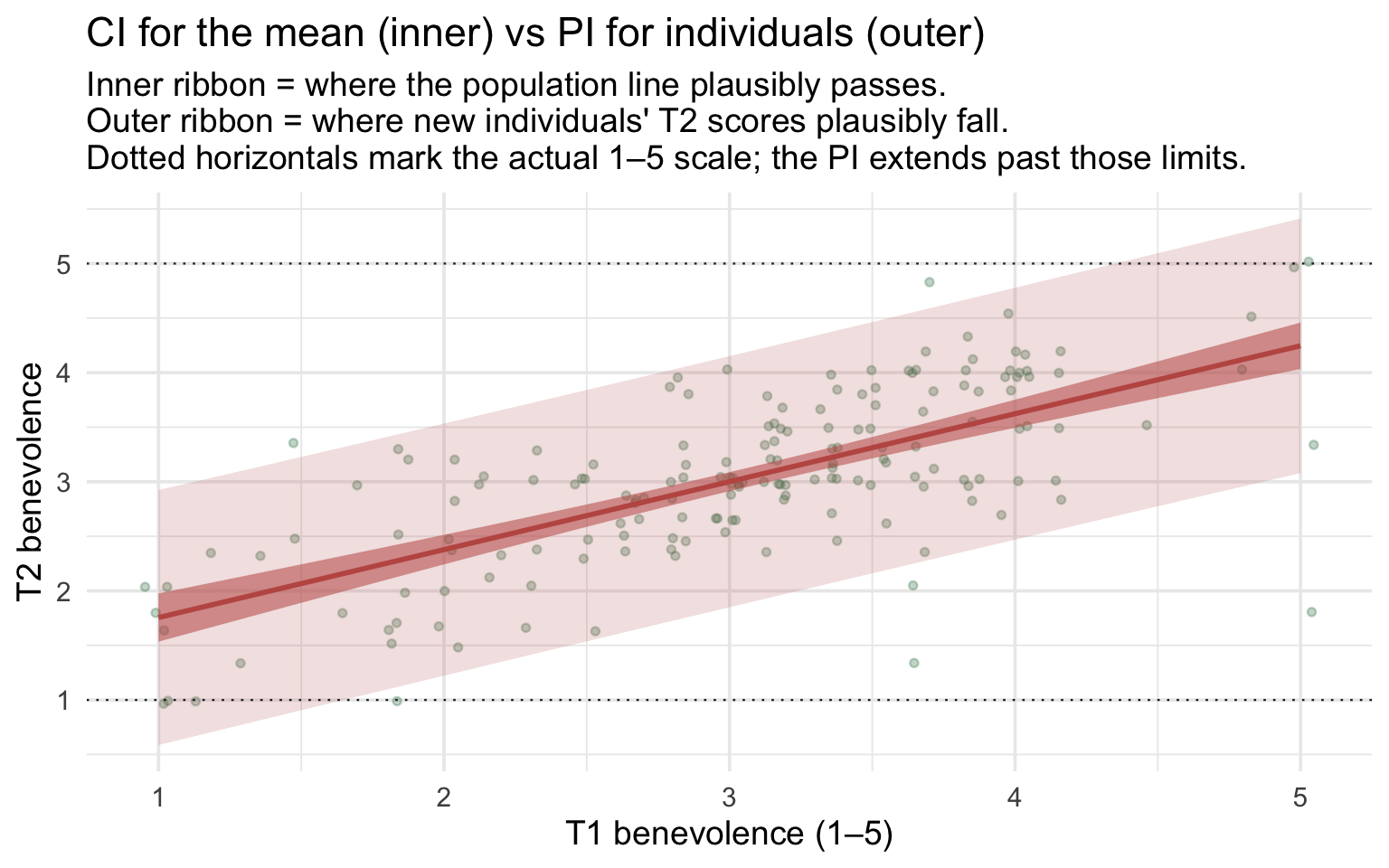
Notice four features:
- The PI ribbon is approximately constant width across the whole range of \(X\). With our 173 data points, the residual SD (\(\sigma\) ≈ 0.58) dominates the PI’s uncertainty at every x; the small “fanning” you might expect at the extremes is mathematically there but invisibly small at this sample size. PI width here ≈ 2.30 benevolence points, regardless of where on the x-axis you stand. That’s close to \(4\sigma\) (2.33): a 95% PI spans about ±\(t^*\sigma\), and with \(t^*\) ≈ 1.97 that’s slightly under the ±2\(\sigma\) person-to-person spread from the \(\sigma\) section. The line’s own uncertainty widens it only slightly.
- The CI ribbon does fan out at the extremes — the classic hourglass shape — but at n = 173 the curvature is gentle. CI width is 0.17 near the data’s center and about 0.43–0.44 at the ends of the scale, roughly 2.5 times wider. The whole band is narrow at n = 173, so the hourglass is easy to miss on this axis; with a smaller sample (say n = 20–50) the band would be wider everywhere and the hourglass easier to see.
- The CI ribbon is much tighter than the PI ribbon at every value of \(X\). With our sample size, the line itself is sharply pinned down. But individual scores scatter around the line with \(\sigma\) ≈ 0.58, and that scatter is what the PI captures.
- The PI is calibrated for future observations conditional on \(x\) — under the fitted model and its assumptions, it should bracket about 95% of fresh draws from the same population, not the in-sample dots specifically. Visually, you can see the PI ribbon brackets roughly 95% of the dots we do have — a quick check — but the real claim is about new participants we haven’t seen yet. The CI ribbon makes a different claim — about the line’s uncertainty — and is not supposed to bracket the dots.
Notice also that the PI extends mathematically below 1 and above 5 — past the actual scale endpoints. That’s because the classical linear-model prediction interval treats future errors as continuous and unbounded; the procedure does not know that the benevolence scale itself stops at 1 and 5. That doesn’t make the fitted line useless, but it reminds us that a linear model can generate predictions that are mathematically possible yet substantively impossible for a bounded outcome. When those boundaries matter strongly, models designed for the outcome’s scale may be preferable: PSY 653 introduces logistic regression for binary outcomes, and more advanced courses take up Poisson-type models for counts and other approaches for bounded or non-Normal outcomes.
A large sample protects the slope’s CI, not the PI. The slope’s CI and the confidence band are about averages, and with a reasonably large sample they hold up well even when the errors aren’t Normal: averaging over many people smooths out the shape of the individual errors, the same reason the central limit theorem lets a sample mean be close to Normal. The PI is different. It describes where one new person’s score will land, the line’s prediction plus that person’s own scatter, so it relies directly on the errors being Normal with the same \(\sigma\) at every T1. More data shrink the line’s uncertainty, but they don’t change how individuals scatter. If that scatter is skewed, or bunched against the 1–5 boundaries, the PI can miss in a predictable direction however large n is. And if the spread grows or shrinks across T1, a single PI width is too wide where people cluster tightly around the line and too narrow where they spread out. Module 12 shows how to check.
Two flavors of regression uncertainty
| Question you’re asking | Tool | Width | What it captures |
|---|---|---|---|
| Where does the line plausibly pass at \(X = x_0\)? | CI for the mean | Narrow, scales with \(1/\sqrt{n}\) | Uncertainty in the line itself |
| What range covers a new individual’s outcome at \(X = x_0\)? | PI for an individual | Wide; shrinks toward about ±2\(\sigma\) as \(n\) grows, never toward 0 | Line uncertainty plus residual scatter |
Use the CI when you’re describing a population-level prediction (e.g., “What is the mean T2 benevolence among control-arm participants with T1 = 3?”). Use the PI when you’re forecasting a specific case (e.g., “What range of T2 should we expect for the next person we screen who scores 3 on T1?”). They answer different questions, and reaching for the wrong one is a common error in applied work.
Inference connections in Parts 2 and 3
The same inferential framework — \(t_\text{obs}\) on the slope, CI on the slope, p-value, and (for predictions) CI for the mean vs PI for the individual — applies to every regression in M10 and beyond. Parts 2 and 3 will make this connection explicit by linking the binary-predictor slope’s t-test to M09’s two-sample t-test (Part 2) and the multi-category predictor’s F-test to M09’s one-way ANOVA (Part 3). M11 will reuse exactly this method for multi-predictor regressions, where each coefficient gets its own t-test and CI — the same method, just applied to coefficients adjusted for the other predictors.
Correlation and standardized regression
A final connection. The Pearson correlation between two variables, \(r\), captures the strength and direction of a linear association on a scale-free \([-1, +1]\) axis:
control |>
  summarize(r_T1_T2 = cor(t1_benevolence, t2_benevolence) |> round(3))
Notice that r² = R² for a simple linear regression: .688² ≈ .473. That’s not coincidence — it’s an algebraic identity for one-predictor regression. Squaring the correlation gives you the proportion of variance shared by the two variables, which is exactly R².
If you standardize both variables (z-score each, so each has mean 0 and SD 1) and refit, the slope of the regression line equals the correlation:
control_z <- control |>
  mutate(
    z_t1 = as.numeric(scale(t1_benevolence)),
    z_t2 = as.numeric(scale(t2_benevolence))
  )

lm(z_t2 ~ z_t1, data = control_z) |>
  tidy(conf.int = TRUE)
The standardized intercept is essentially zero (the line passes through the origin of the z-scaled cloud); the standardized slope equals \(r\). So \(r\) is the regression slope on the standardized scale — a property that motivates why \(r\) is sometimes called the standardized slope (some books write it as \(\beta\) — a different use of the letter from the population slope \(\beta_1\)).
The two slopes are not the same number. The unstandardized slope \(b_1\) = 0.623 is in the units of the data — the predicted T2 difference, in scale points, between people one T1 point apart. The standardized slope \(r\) ≈ .688 is unit-free — the predicted T2 difference, in SDs, between people one SD apart on T1. They convey different practical information, and which one to report depends on whether your audience cares about the original scale (then \(b_1\)) or about cross-study comparability (then \(r\)). One caution on comparability: \(r\) also depends on how spread out \(X\) is in each sample. A study that recruits only a narrow range of baseline scores will show a smaller \(r\) (and R²), even if the line and \(\sigma\) are exactly the same.
TipGoing further — a confidence interval for r
The standardized regression above prints a 95% CI for its slope, [.578, .797]. That interval is centered on r and reaches the same distance on both sides. It is not the right interval for the population correlation, \(\rho\), for two reasons:
- \(r\) is bounded at −1 and +1. When the true correlation is far from 0, the sampling distribution of \(r\) gets squeezed against the nearer bound and becomes lopsided. A symmetric “estimate ± \(t^*\) × SE” interval misdescribes that shape, and for a strong enough correlation it can even run past 1.
- Standardizing used the sample’s own SDs, which the regression then treats as if they were known.
The standard fix is Fisher’s z transformation. Convert \(r\) to \(z = \tanh^{-1}(r) = \tfrac{1}{2}\ln\!\left[\frac{1 + r}{1 - r}\right]\), a scale with no bounds on which the sampling distribution is close to Normal, with \(SE \approx 1/\sqrt{n - 3}\). Build the 95% CI on that scale, then convert both ends back with \(r = \tanh(z)\). The back-converted interval always stays inside [−1, 1], and it is asymmetric: it reaches farther toward 0 than away from it. cor.test() does all of this for you:
cor.test(~ t1_benevolence + t2_benevolence, data = control) |>
  tidy()
For the Hong Kong control arm, r = .688, 95% CI [.600, .759]. The lower end sits .088 below r; the upper end sits only .071 above it. When the correlation itself is the result you report, use this interval rather than the standardized slope’s.
APA-style reporting
APA-style reporting · Simple Linear Regression (continuous predictor)
Among 173 Hong Kong control-arm participants, baseline benevolence was positively associated with 2-week follow-up benevolence, b = 0.623, SE = 0.050, 95% CI [0.523, 0.722], t(171) = 12.39, p < .001. Participants whose baseline benevolence was one point higher were predicted to score 0.623 points higher at follow-up. Baseline benevolence accounted for 47.3% of the variance in follow-up benevolence (R² = .473, σ = 0.581).
Note the structure: b with SE and 95% CI → t with df → p → plain-language slope interpretation → R² → residual SE.
Part 2 — A binary categorical predictor
First, a prerequisite: store categorical predictors as factors
Everything in Parts 2 and 3 rests on how R stores the categorical variable. The safest choice is a factor, R’s type for a categorical variable. A factor carries two things a plain column does not — the set of levels (the categories) and their order, and that order matters here because lm() treats the first level as the reference group.
Make categorical predictors factors explicitly. R can automatically treat a character (text) variable as categorical in a regression, but converting it to a factor yourself lets you inspect and control its levels and its reference group. Numeric category codes are different: without conversion to a factor, R treats them as a quantitative predictor and fits a single numeric slope — exactly right for a 0/1 dummy you built on purpose, and exactly wrong for codes like sites numbered 1 through 6.
Check what you have. class() reports the type, and levels() lists the categories in order:
reach |> pull(treat) |> class()[1] "factor"reach |> pull(treat) |> levels()[1] "Control" "Treatment"Our course datasets arrive ready to use, so treat and site are already factors. Data you collect yourself usually won’t be.
Make a factor. factor() converts a character or numeric column. On its own it sorts the levels alphabetically; the levels = argument sets the order you want, and whichever level you list first becomes the reference:
dose_text <- c("Low", "High", "Medium", "Low")   # e.g. a column read straight from a CSV
class(dose_text)
[1] "character"factor(dose_text) |> levels() # alphabetical by default[1] "High" "Low" "Medium"factor(dose_text, levels = c("Low", "Medium", "High")) |>
levels() # the order you choose[1] "Low" "Medium" "High" Inside a data frame, that conversion goes in a mutate(): mutate(arm = factor(arm, levels = c("Control", "Treatment"))). To change the reference of a factor you already have, use fct_relevel() — Part 3 does exactly that. And for SPSS-style labelled data, where the categories are stored as numeric codes with value labels attached, haven::as_factor() promotes those labels into levels in one step (the M05 bonus lab on labelled data covers that case).
Why it matters. If a grouping variable stays numeric — sites coded 1 through 6, say — lm() reads the codes as a measurement and fits one slope through them instead of building dummies. No error, no warning, just the wrong model. For a deeper treatment of factors, see Chapter 16 (Factors) of R for Data Science.
What kind of question is this? Part 2 is built from a randomized experiment, so treatment assignment itself can support a causal comparison: participants were randomly assigned to the immediate workbook or the waitlist control.
There is one complication. Our classroom analysis uses only participants with an observed T2 benevolence score. Follow-up completion happens after randomization, so restricting the analysis to complete cases can weaken the protection randomization originally gave us. The concern is not simply that dropout rates might differ between arms. It’s that, within an arm, who completes the follow-up could be related to their benevolence; then the participants we analyze may no longer be a fair comparison of the two randomized groups.
So read this regression as the unadjusted treatment-group contrast among participants with observed follow-up data, with a causal interpretation that additionally depends on assumptions about follow-up missingness. Random assignment is what distinguishes this from an ordinary observational between-group association; the complete-case restriction is why we keep some caution. (The published REACH analysis did not use this complete-case model: it used multiple imputation and an intention-to-treat model that included site.)
M11 will fit the stronger baseline-adjusted regression. In substantive trial work, missing outcome data would also deserve a fuller intention-to-treat and missing-data strategy, not an afterthought.
Scaling up to the full sample
In Part 1 we worked with the Hong Kong control arm — n = 173 — because the smaller sample made the geometry of regression visible (residual segments readable, bootstrap lines fanning out at the extremes). With the conceptual steps anchored, we now move beyond the Hong Kong control arm to the full REACH dataset (both Treatment and Control, all six sites). For the treatment comparison in this Part, we analyze the participants with an observed T2 score; for the baseline site comparison in Part 3, we can use all 4,598 participants. Three things change:
- Sample size jumps more than 20-fold. Standard errors shrink (roughly in proportion to \(1/\sqrt{n}\)); confidence intervals become much narrower than they were on Hong Kong’s n = 173.
- The coefficient now compares randomized treatment groups. Including both arms lets us estimate the difference in follow-up benevolence between participants assigned to Treatment and to Control; the missing-follow-up caveat above still applies.
- Categorical predictors enter the model. Treatment is a binary factor (Part 2); site is a 6-level factor (Part 3). The dummy coding you’ll meet in this Part scales into M11 unchanged.
The same lm() syntax we used on Hong Kong control covers the full-sample analyses below — what changes is just which rows go into the model and which kind of predictor sits on the right side of the formula.
Our second regression switches predictors: instead of a continuous predictor (baseline benevolence), we use a binary categorical predictor (treatment condition). The research question is our benevolence version of the central question REACH was designed to answer (the paper’s own outcome was the combined unforgiveness score):
Did random assignment to the immediate REACH workbook produce higher 2-week follow-up benevolence than waitlist control?
For this question we use all participants with an observed follow-up score — both control and treatment arms — with t2_benevolence as the outcome and treat as the predictor. We drop participants missing a follow-up score (complete-case analysis):
analysis <- reach |>
  drop_na(t2_benevolence)

analysis |>
  group_by(treat) |>
  summarize(
    n = n(),
    M = mean(t2_benevolence) |> round(3),
    SD = sd(t2_benevolence)   |> round(3)
  )
The sample has 2,057 control participants and 1,908 treatment participants with follow-up. Treatment-arm mean follow-up benevolence (3.72) is visibly higher than the control-arm mean (3.20) — a difference of about 0.52 points on the 1–5 scale. We’ll formalize that comparison via regression.
How does a regression handle a categorical predictor?
A regression slope is “the predicted difference in \(y\) between cases one unit apart on \(x\).” That’s straightforward when \(x\) is continuous — but what does “one unit apart” mean for a categorical predictor like treat, whose values are the strings Control and Treatment? The trick is to turn the category into a 0/1 numeric column — a dummy indicator. Once the predictor is 0/1, “one unit apart” has a concrete meaning: one case in each category.
There are two ways to build the dummy in R, and they give exactly the same answer.
Route 1 — Build it by hand with mutate() + case_when(). Pick a reference category (the level coded as 0) and a contrast category (coded as 1):
analysis_dummy <- analysis |>
  mutate(treat_dummy = case_when(
    treat == "Control"   ~ 0,
    treat == "Treatment" ~ 1
  ))

analysis_dummy |> select(treat, treat_dummy) |> slice_head(n = 4)
Now treat_dummy is a numeric 0/1 column we can put in lm() just like any other numeric predictor.
Route 2 — Hand the factor to lm() directly. R does the dummy coding automatically: it uses the first level of the factor as the reference (coded 0) — here Control — and gives the other level a coefficient with the level’s name appended. (A factor built from raw character strings usually stores its levels alphabetically, so the reference is often the alphabetically-first level; but if the levels were set deliberately, R honors that order — so it’s safest to set the reference explicitly with fct_relevel().)
treat_mod <- lm(t2_benevolence ~ treat, data = analysis)
treat_mod |> tidy() |> select(term, estimate)
The coefficient name treatTreatment tells you which level is the contrast (Treatment), and the absence of a treatControl coefficient tells you which level is the reference (Control, coded 0). Behind the scenes, R built the same 0/1 column you built manually with case_when(). The two routes return identical coefficients — the factor route is just a shortcut.
You can read R’s coding scheme directly with contrasts():
analysis |> pull(treat) |> contrasts() Treatment
Control 0
Treatment 1The single column — named Treatment — is the 0/1 dummy: Control maps to 0 (the reference), Treatment to 1.
Route 2 relies on R treating the variable as categorical. lm() builds the dummy for treat here because the data frame stores it as a factor — R’s type for categorical variables, which carries the set of levels and their order. Our course datasets arrive with treat and site already stored as factors, but in your own data, check before you fit, because the two common alternatives behave differently. A character column ("Control" / "Treatment" as plain text) is silently converted to a factor with alphabetical levels, so you get the dummies but no say over the reference. A numeric code column is the one to watch: for a binary 0/1 variable that’s exactly Route 1 and works fine, but with three or more categories (sites coded 1–6, say) lm() treats the codes as a continuous measure and fits a single slope through them instead of building dummies — no error, no warning, just the wrong model. The fix is the one-line factor() conversion from the box at the top of this Part.
Switching the reference group. If you’d rather the intercept be the Treatment mean and the slope be the (Control − Treatment) difference, fct_relevel() reorders the factor: analysis |> mutate(treat = fct_relevel(treat, "Treatment")). Same model, same fit, same R² — only the parameterization changes (the intercept changes, and the slope’s sign flips). Reference-group choice is entirely a reporting decision, not a statistical one.
Plug in the equation to recover both group means
Once we have the 0/1 encoding, the regression equation is
\[\widehat{\text{T2}}_i \;=\; b_0 \;+\; b_1 \cdot \text{treat}\_\text{dummy}_i\]
The key step is to plug in the dummy values for each group:
- Control participants have \(\text{treat}\_\text{dummy} = 0\), so \(\widehat{\text{T2}} = b_0 + b_1 \cdot 0 = b_0\). The intercept is the Control group mean.
- Treatment participants have \(\text{treat}\_\text{dummy} = 1\), so \(\widehat{\text{T2}} = b_0 + b_1 \cdot 1 = b_0 + b_1\). The intercept plus the slope is the Treatment group mean.
Subtracting the two gives the slope back: \(b_1 = (b_0 + b_1) - b_0 = M_{\text{Treatment}} - M_{\text{Control}}\). So here is the key insight of dummy coding: with a binary predictor, the intercept is the reference-group mean and the slope is the between-group mean difference. The plug-in arithmetic is the proof.
Visualize the data
Before fitting, look at the data — three pictures, one question: how far apart do the two groups’ centers sit, and how much do the individuals overlap? Hold both halves of that question as you look, because the regression is about to estimate the first half while the second half stays stubbornly large.
First, the violin-and-box view. The violin shows each group’s distribution shape, the box marks the IQR, and the gold dot is the group mean — the dots are where your eye should go first.
Show the code that built this figure
analysis |>
  ggplot(aes(x = treat, y = t2_benevolence, fill = treat)) +
  geom_violin(alpha = 0.30, color = NA) +
  geom_boxplot(width = 0.15, fill = "white", outlier.alpha = 0.30) +
  stat_summary(fun = mean, geom = "point", shape = 21, size = 3.5,
               fill = "#AD872B", color = "#AD872B") +
  scale_fill_manual(values = c("Control" = "#3A8055", "Treatment" = "#4E5EAA"),
                    guide = "none") +
  scale_y_continuous(breaks = 1:5) +
  labs(
    x = NULL, y = "T2 benevolence (1–5)",
    title = "T2 benevolence by treatment condition",
    subtitle = "Gold dot = group mean. The treatment cloud sits visibly higher."
  )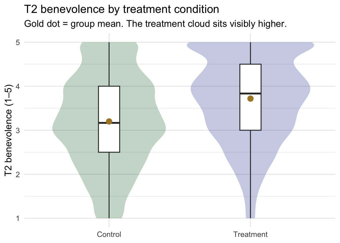
The treatment cloud’s center lies higher than the control cloud’s center — by roughly half a benevolence point. The distributions overlap a great deal, so the difference is not “everyone in treatment ends higher than everyone in control.” It’s a shift in the average.
A density plot sharpens the same story by overlaying the two smoothed distributions on a single x-axis — watch how much territory the two curves share even though one peak sits clearly to the right of the other:
Show the code that built this figure
analysis |>
  ggplot(aes(x = t2_benevolence, fill = treat)) +
  geom_density(alpha = 0.55, color = NA) +
  scale_fill_manual(values = c("Control" = "#3A8055", "Treatment" = "#4E5EAA")) +
  scale_x_continuous(breaks = 1:5) +
  labs(
    x = "T2 benevolence (1–5)", y = "Density", fill = "Condition",
    title = "Where the two distributions sit on the scale",
    subtitle = "Same x-axis (T2 benevolence); two overlapping smoothed distributions."
  ) +
  theme(legend.position = "top")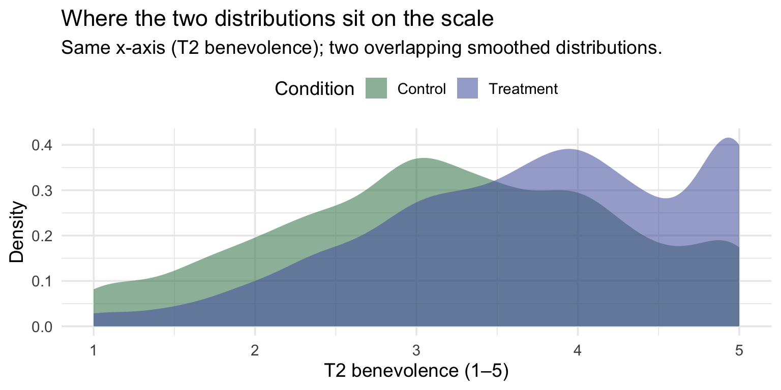
Finally, a jittered scatter with the group means overlaid — the least-processed view, and the one to check the other two against: every participant as a dot, with the group mean marked as a gold disk:
Show the code that built this figure
analysis |>
  ggplot(aes(x = treat, y = t2_benevolence, color = treat)) +
  geom_jitter(width = 0.18, height = 0.05, alpha = 0.18, size = 1.0) +
  stat_summary(fun = mean, geom = "point", shape = 21, size = 4,
               fill = "#AD872B", color = "#AD872B") +
  scale_color_manual(values = c("Control" = "#3A8055", "Treatment" = "#4E5EAA"),
                     guide = "none") +
  scale_y_continuous(breaks = 1:5) +
  labs(
    x = NULL, y = "T2 benevolence (1–5)",
    title = "Every participant + the group means",
    subtitle = "Gold circles = group means.\nDots are jittered horizontally so overlapping respondents are visible."
  )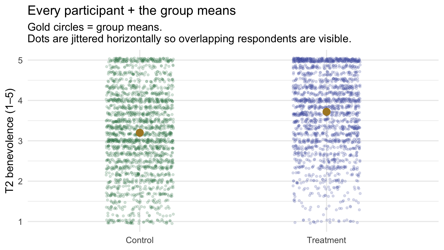
Fit the model
treat_mod <- lm(t2_benevolence ~ treat, data = analysis)
treat_mod |> tidy(conf.int = TRUE)
treat_mod |> glance()Reading off:
- Intercept \(b_0\) = 3.200. The model’s predicted T2 benevolence for a Control participant (\(\text{treatTreatment} = 0\)). And it’s exactly the Control group mean we computed in the descriptive table above (3.200). ✓
- Slope \(b_1\) = 0.519 (95% CI [0.456, 0.583]). The change in predicted T2 benevolence going from Control → Treatment. And it’s exactly the mean difference (Treatment − Control = 3.719 − 3.200 = 0.519). ✓
The slope’s 95% CI runs from 0.46 to 0.58, entirely above zero: participants assigned to the workbook scored about half a benevolence point higher than controls at 2 weeks (among those with follow-up data), and the data give strong evidence that the population difference is positive.
The model fit summaries:
- R² = .061 — treatment condition accounts for 6.1% of the variation in T2 benevolence. That sounds small, but values like this are common for a single-predictor treatment comparison in psychology, and it corresponds to a medium standardized difference (the Cohen’s d computed below). Most of the person-to-person variation (idiosyncratic life events, day-to-day mood, baseline differences) remains within the two groups.
- \(\sigma\) = 1.017 — the residual scatter is on the scale of about a full benevolence point. Compare to SD of T2 benevolence in the analysis sample (1.049): the reduction is small, because treat alone accounts for only a small share of the outcome’s variation. M11 will show what happens when we add baseline benevolence to the model.
This unadjusted model is for learning, not the trial’s final analysis. Regressing t2_benevolence on treat alone is the cleanest way to see dummy coding — but it isn’t the strongest way to estimate the treatment effect. A more powerful RCT analysis would adjust for baseline benevolence (and likely site), absorbing the outcome variation that baseline accounts for and tightening the treatment-effect estimate. That baseline-adjusted model is exactly the multiple regression you’ll build in Module 11.
The slope, geometrically: rise over run on a 0/1 axis
Part 1 introduced the slope as rise over run — the difference in \(\hat{y}\) between cases one unit apart on \(x\). With a continuous predictor, “one unit” was just one unit of T1 benevolence. With a binary predictor, the dummy goes from \(0\) (Control) to \(1\) (Treatment), so the run is exactly 1 by construction. That makes the slope’s geometry especially clean: the slope IS the mean difference, because the run is fixed at 1 and the rise is the gap between group means.
Here’s that picture, with the gold mean dots connected by the regression line and the rise/run annotated explicitly:
Show the code that built this figure
group_means <- analysis |>
  group_by(treat) |>
  summarize(M = mean(t2_benevolence))

ctrl_M_y <- group_means |> filter(treat == "Control") |> pull(M)
trt_M_y  <- group_means |> filter(treat == "Treatment") |> pull(M)
rise_val <- trt_M_y - ctrl_M_y

ggplot(group_means, aes(x = treat, y = M)) +
  # the regression line connecting the two group means (drawn once via annotate)
  annotate("segment", x = "Control", xend = "Treatment",
           y = ctrl_M_y, yend = trt_M_y,
           color = "#1C2433", linewidth = 0.9) +
  # run (horizontal dashed) and rise (vertical dashed) in rose
  annotate("segment", x = "Control", xend = "Treatment",
           y = ctrl_M_y, yend = ctrl_M_y,
           color = "#C05852", linewidth = 1.2, linetype = "dashed") +
  annotate("segment", x = "Treatment", xend = "Treatment",
           y = ctrl_M_y, yend = trt_M_y,
           color = "#C05852", linewidth = 1.2, linetype = "dashed") +
  # mean dots
  geom_point(aes(color = treat), size = 5) +
  geom_text(aes(label = sprintf("%.2f", M)), vjust = -1.0,
            size = 4, color = "#1C2433") +
  # rise/run labels — plain text annotations, no box
  annotate("text", x = 1.5, y = ctrl_M_y - 0.04,
           label = "run = 1",
           color = "#C05852", fontface = "bold", size = 4) +
  annotate("text", x = 1.5, y = ctrl_M_y - 0.10,
           label = "(one step on the dummy: Control → Treatment)",
           color = "#C05852", size = 3.2) +
  annotate("text", x = 2.06, y = (ctrl_M_y + trt_M_y)/2,
           label = sprintf("rise = %.3f", rise_val),
           color = "#C05852", fontface = "bold", size = 4, hjust = 0) +
  annotate("text", x = 2.06, y = (ctrl_M_y + trt_M_y)/2 - 0.06,
           label = "(treatment mean − control mean)",
           color = "#C05852", size = 3.2, hjust = 0) +
  scale_color_manual(values = c("Control" = "#3A8055", "Treatment" = "#4E5EAA"),
                     guide = "none") +
  labs(
    x = NULL, y = "T2 benevolence",
    title = "The slope on a 0/1 dummy axis",
    subtitle = sprintf(
      "Run = 1 (Control → Treatment is one unit of the dummy).\nRise = %.3f = the slope = the mean difference.",
      rise_val)
  ) +
  # room above the Treatment dot for its label, and to the right for the rise labels
  scale_y_continuous(expand = expansion(mult = c(0.12, 0.15))) +
  scale_x_discrete(expand = expansion(add = c(0.4, 1.05)))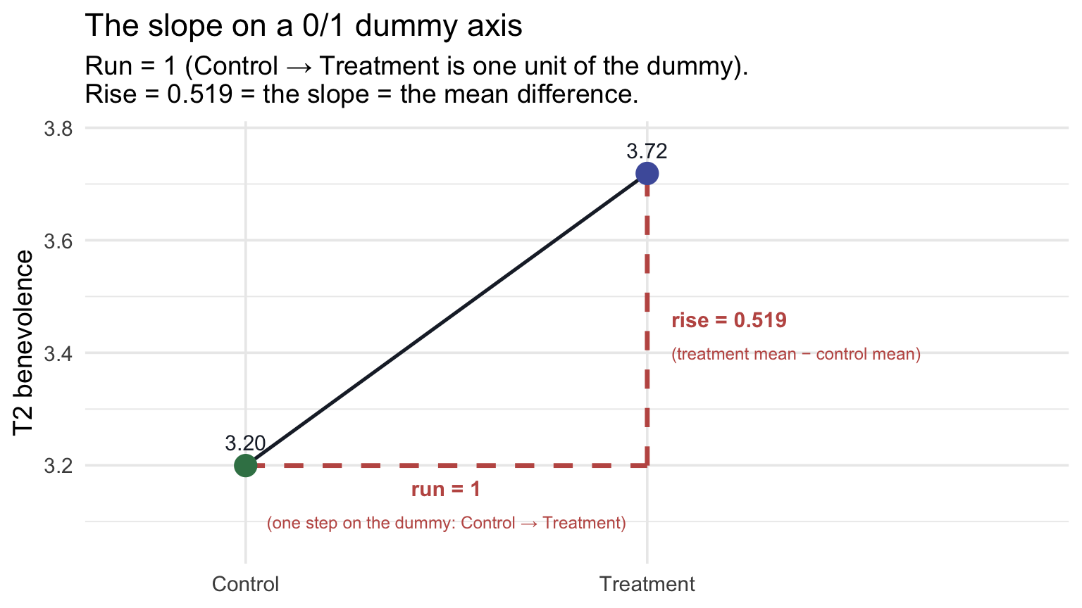
This is the same visualization Part 1 used to introduce the slope on a continuous axis — except the run is now mechanically 1 (by the dummy coding), so the slope and the mean difference are the same number by construction.
Why the slope is the mean difference (when the predictor is binary)
The dummy-coded predictor has exactly two values: 0 and 1. So two cases one unit apart on it are always one Control participant (0) and one Treatment participant (1). The slope, the predicted difference in \(y\) between cases one unit apart on \(x\), is therefore the predicted difference between a Treatment participant and a Control participant. That’s the mean difference. The intercept \(b_0\) is the predicted \(y\) at \(x = 0\) (the Control mean); the predicted \(y\) at \(x = 1\) is \(b_0 + b_1\) (the Treatment mean). Subtracting: \(b_1\) = Treatment mean − Control mean, exactly.
Connection to the two-sample t-test (M09 Test 1)
In M09 Test 1 we ran a two-sample t-test on the Hofman boulder data — testing whether two groups had the same population mean. The procedure had a separate name and a separate output. And yet: the slope of lm(y ~ group) is the same number as the mean difference a two-sample t-test estimates, and lm(y ~ group)’s slope \(t_\text{obs}\) is the same number that the standard (Student’s) equal-variance version of that test reports. M09 built the standard (Student’s) version by hand and showed Welch’s t-test beside it. Welch’s version relaxes the equal-variance assumption and is R’s default; the OLS regression’s \(t_\text{obs}\) matches the standard version, not Welch’s. The two are closely related but not interchangeable.
To make the connection literal, run an equal-variance two-sample t-test on our REACH data with infer::t_test() and compare:
analysis |>
  t_test(response = t2_benevolence,
         explanatory = treat,
         order = c("Treatment", "Control"),
         var.equal = TRUE)
Compare to the lm() output above: the two-sample test’s \(t_\text{obs}\), its df, and its p-value are identical to the regression’s slope-on-treat \(t_\text{obs}\), slope df, and p. The mean-difference (estimate) and its 95% CI are identical too. They are not coincidentally similar; they are the same procedure with a different name. Default infer::t_test() returns Welch’s version (var.equal = FALSE); we pass var.equal = TRUE here to match the OLS regression’s pooled-variance assumption exactly. With near-equal group sizes and SDs, the Welch and standard (Student’s) versions differ only slightly (here, by about 0.04 on the t-statistic), but the exact match to lm() comes from var.equal = TRUE. This exact equivalence is a mathematical bridge, not a recommendation to abandon Welch’s test: when group variances differ, Welch’s t-test (R’s default, shown beside the standard version in M09) or heteroscedasticity-robust regression SEs (M12; standard errors that allow unequal residual spread) remain the more defensible inferential tools.
That’s the regression-as-parent-framework point M09’s Looking ahead section previewed: when the predictor is a binary categorical variable, an SLR is the standard (Student’s) two-sample t-test. The advantage of writing it as a regression is that you can easily generalize: add a continuous covariate (M11), add an interaction (PSY 653), or swap to a categorical predictor with more than two levels (Part 3, immediately below). Each generalization is a tiny extension of the same lm() syntax.
Effect size: Cohen’s d
For categorical predictors with two levels, the conventional effect-size complement to the slope is Cohen’s d — the standardized mean difference. From effectsize::cohens_d():
# cohens_d() subtracts in factor-level order. Put Treatment first, so d is
# Treatment - Control, the same direction as the slope.
analysis_trt_first <- analysis |>
  mutate(treat = fct_relevel(treat, "Treatment"))

cohens_d(t2_benevolence ~ treat, data = analysis_trt_first)
Start with the raw units: the workbook group scored about 0.52 of a point higher on the 1–5 scale. Cohen’s d rescales that same gap by the pooled SD, and that pooled SD is exactly the model’s \(\sigma\) (1.017), so here d = \(b_1 / \sigma\) = 0.511 (95% CI [0.447, 0.574]). Because we put Treatment first, d is Treatment − Control, the same direction as the slope. The CI is fully bounded away from zero. Cohen’s rough benchmarks would call the standardized size medium, but, as with R², the more useful question is what a gap of that size means for this outcome.
APA-style reporting
APA-style reporting · Simple Linear Regression (binary categorical predictor)
Among 3,965 participants completing the 2-week follow-up, treatment-condition participants reported higher follow-up benevolence (M = 3.72, SD = 0.98, n = 1,908) than control-condition participants (M = 3.20, SD = 1.05, n = 2,057), b = 0.519, SE = 0.032, 95% CI [0.456, 0.583], t(3963) = 16.07, p < .001, Cohen’s d = 0.51, 95% CI [0.45, 0.57]. Treatment condition accounted for 6.1% of the variance in follow-up benevolence (R² = .061, σ = 1.017).
Note the structure: group descriptives → slope (= mean difference) with SE and 95% CI → t with df → p → effect size (Cohen’s d) with CI → R² → residual SE.
Part 3 — A multi-category categorical predictor
Still one predictor? Yes: site is one predictor term, but its six levels require five coefficients. R represents that one factor with five dummy-coded columns behind the scenes, so the fitted model carries one intercept plus five slopes. You can think of it as a single-factor linear model: the same OLS framework as SLR, now represented by several dummy variables. (Texts differ on whether to call this “simple” regression; many reserve that name for one numerical predictor.) The model estimates six regression coefficients — one intercept and five site contrasts — which together recover the six site means. The omnibus F-test therefore has 5 numerator degrees of freedom (one per site contrast) and n − 6 denominator degrees of freedom.
What kind of question is this? Part 3 is descriptive/comparative — there’s no random assignment to “site” (people are nested in their study sites) and no causal claim being made. We’re describing the between-site differences in baseline benevolence as they exist, before the intervention rolls out. The regression coefficients quantify those differences but don’t say why they exist; that would require an entirely different study design.
Our third regression introduces a categorical predictor with more than two levels. The research question:
Do the six study sites differ in baseline benevolence?
Notice that the outcome here is T1 benevolence, measured before treatment could have had any effect. This is therefore not a treatment-effect analysis. Instead, we’re using the linear-model framework to describe another important feature of a multisite dataset: how much baseline benevolence differs across the six study sites.
A multisite randomized trial does not require the sites themselves to have identical baseline means. Participants at different sites may come from very different populations and contexts. What randomization is designed to balance is the two arms (Treatment vs Control) within each site, not Colombia against Hong Kong or Indonesia against Ukraine. So our question here is descriptive, and it gives us a natural way to learn how regression handles a categorical predictor with more than two levels.
For this analysis we use the full sample (we don’t need participants to have completed T2):
reach |>
  group_by(site) |>
  summarize(
    n = n(),
    M = mean(t1_benevolence) |> round(3),
    SD = sd(t1_benevolence)   |> round(3)
  )
The sample has 4,598 participants across six sites. The site means range from 2.963 to 3.391 — a spread of about 0.43 benevolence points. The regression will quantify those between-site differences and their sampling uncertainty.
Why one slope isn’t enough
A single slope says “the predicted difference in \(Y\) between cases one unit apart on \(X\).” That’s well-defined when \(X\) is continuous (two people one point apart on T1) and when \(X\) is binary (a Control and a Treatment participant are one unit apart on the dummy). But what does “one unit apart on site” mean? Colombia → Hong Kong? Hong Kong → Indonesia? There’s no inherent ordering, so there’s no single slope.
The fix is multiple dummies. With six sites, R creates five 0/1 indicators — one fewer than the number of categories. The convention is “\(k - 1\) dummies for \(k\) categories”:
- One category becomes the reference (omitted from the dummies — it’s the “base case”).
- Each of the other five gets its own dummy: 1 if the participant is in that site, 0 otherwise.
So a participant in Indonesia has \(\text{site}_{\text{Indonesia}} = 1\), and zeros for all four other site dummies. A participant in Colombia (the reference site) has 0 on all five site dummies, so the reference category is identified by the absence of any non-reference-site indicator.
Letting lm() build the dummies
Hand the factor to lm(). R builds the five dummies automatically when we put the site factor in the formula (one predictor variable, five site coefficients) — the first factor level becomes the reference, and the other five get coefficients named siteHong Kong, siteIndonesia, and so on. So although site appears as just one variable in the formula, R represents its six categories with five dummy predictors: the model has one explanatory variable but several coefficients. That prepares us for M11, where several explanatory variables appear together. This is what we’ll use throughout Part 3 because it’s much more compact than carrying five hand-built columns (the folded box below shows how you’d build them) through a tidyverse pipeline. As in Part 2, the automatic dummy-building happens because site is stored as a factor: if your own grouping variable arrived as text or as numeric codes, you’d convert it first with factor(), as the box at the top of Part 2 shows.
Set the reference on purpose. Everything that follows reads each coefficient as “that site minus Colombia,” so the model has to agree. Colombia happens to be the first level already, but rather than rely on that (as in Part 2, a factor’s order is alphabetical only when nobody set it deliberately), we make it the reference explicitly with fct_relevel() before fitting anything. The arguments are the variable, then the level you want to assign to the reference group — fct_relevel() moves that level to the front of the level order, and lm() always uses the first level as the reference:
reach <- reach |>
  mutate(site = fct_relevel(site, "Colombia"))   # Colombia = the reference site

reach |> pull(site) |> levels()                 # the first level listed is the reference
[1] "Colombia" "Hong Kong" "Indonesia" "South Africa"
[5] "Ukraine (Realis)" "Ukraine (UISA)" Now the teaching text and the fitted model are guaranteed to line up.
TipGoing further — building the five site dummies by hand
With more categories the case_when() syntax gets verbose, so we typically build one indicator at a time:
analysis_site_dummies <- reach |>
  mutate(
    site_HK = if_else(site == "Hong Kong",        1, 0),
    site_IN = if_else(site == "Indonesia",        1, 0),
    site_SA = if_else(site == "South Africa",     1, 0),
    site_UR = if_else(site == "Ukraine (Realis)", 1, 0),
    site_UU = if_else(site == "Ukraine (UISA)",   1, 0)
  )

analysis_site_dummies |>
  select(site, site_HK, site_IN, site_SA, site_UR, site_UU) |>
  slice_head(n = 6)
A Colombia participant has all five dummies equal to 0; a Hong Kong participant has site_HK = 1 and the rest 0. We could feed those five 0/1 columns to lm() just like any other numeric predictors.
The regression equation, with the five dummies in place, is
\[\widehat{\text{T1}}_i \;=\; b_0 + b_{HK} \cdot \text{site}_{HK,i} + b_{IN} \cdot \text{site}_{IN,i} + b_{SA} \cdot \text{site}_{SA,i} + b_{UR} \cdot \text{site}_{UR,i} + b_{UU} \cdot \text{site}_{UU,i}\]
with \(b_0\) the Colombia mean (the reference) and each other \(b\) the difference between that site’s mean and Colombia’s (HK = Hong Kong, IN = Indonesia, SA = South Africa, UR = Ukraine (Realis), UU = Ukraine (UISA)).
Plug in the dummies to recover any site’s mean
Same key step as the binary case, repeated five times. Set the dummy for the site of interest to 1, leave the others at 0, and add to the intercept:
- Colombia (reference): all five dummies are 0, so \(\widehat{\text{T1}} = b_0\).
- Hong Kong: \(\text{site}_{HK} = 1\), others 0, so \(\widehat{\text{T1}} = b_0 + b_{HK}\).
- …and so on for the other four sites — one dummy switched on, that site’s coefficient added to the intercept.
Six site means, recovered from one intercept and five slopes. The intercept anchors the reference; each slope tells you how far that site’s mean sits above or below the reference.
Choosing a different reference group. We picked Colombia only for convenience; no site has a special status in this question. Sometimes, though, you want the intercept to be a meaningful, theoretically motivated “baseline” category — perhaps the site with the largest sample, or a site that’s the historical reference for prior REACH research. To set the reference explicitly:
reach |>
  mutate(site = fct_relevel(site, "Hong Kong")) |>
  lm(t1_benevolence ~ site, data = _)
Same fit, same R², same predicted means — but the intercept is now the Hong Kong mean and each of the five slopes is “site mean − Hong Kong mean.”
Visualize the data
Show the code that built this figure
grand_mean <- reach |> pull(t1_benevolence) |> mean()

reach |>
  ggplot(aes(x = site, y = t1_benevolence, color = site)) +
  geom_jitter(width = 0.18, height = 0.05, alpha = 0.10, size = 1.2) +
  stat_summary(fun = mean, geom = "point", shape = 21, size = 4.5,
               fill = "#AD872B", color = "#1C2433", stroke = 1) +
  geom_hline(yintercept = grand_mean, color = "#C05852",
             linetype = "dashed", linewidth = 0.7) +
  scale_color_manual(values = c(
    "Colombia" = "#348C9E",
    "Hong Kong" = "#C05852",
    "Indonesia" = "#AD872B",
    "South Africa" = "#4E5EAA",
    "Ukraine (Realis)" = "#945297",
    "Ukraine (UISA)" = "#3A8055"
  ), guide = "none") +
  scale_y_continuous(breaks = 1:5) +
  labs(
    x = NULL, y = "T1 benevolence (1–5)",
    title = "Baseline benevolence by site",
    subtitle = sprintf("Gold dots = site means; rose dashed line = grand mean (%.2f)", grand_mean)
  ) +
  theme(axis.text.x = element_text(angle = 30, hjust = 1))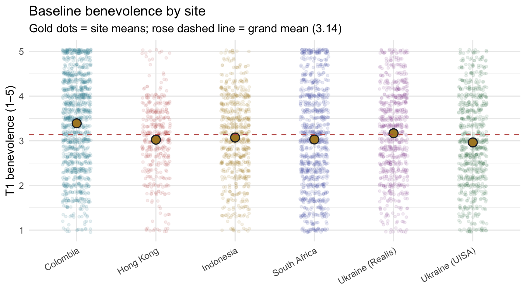
Visually, Colombia sits noticeably higher than the other five sites, and the three other non-Ukraine sites (Hong Kong, Indonesia, South Africa) cluster within a tight band below it; Ukraine (Realis) lands between Colombia and that band, and Ukraine (UISA) sits at the bottom. Whether the visible spread reflects population differences or sampling fluctuation around a common mean — that’s what the regression formalizes.
Fit the model
site_mod <- lm(t1_benevolence ~ site, data = reach)
site_mod |> tidy(conf.int = TRUE)
site_mod |> glance()Six rows in the tidy() output — the intercept plus five site dummies. Read them in pairs:
- Intercept \(b_0\) = 3.391. The Colombia mean. Compare to the descriptive table: yes, Colombia’s M is 3.391. ✓
- siteHong Kong \(b_{HK}\) = -0.366. Hong Kong’s mean is lower than Colombia’s by about 0.37 of a benevolence point. Compare: Hong Kong’s M = 3.024; Colombia + slope = 3.024. ✓
- siteIndonesia = -0.318. Compare: Indonesia’s M = 3.072; Colombia + slope = 3.072. ✓
- siteSouth Africa = -0.361. Compare: South Africa’s M = 3.029; Colombia + slope = 3.029. ✓
- siteUkraine (Realis) = -0.223. Smallest gap.
- siteUkraine (UISA) = -0.428. Largest negative gap.
All five 95% CIs lie entirely below zero: compared with Colombia, each of the other five estimated site means is lower. These are five unadjusted reference contrasts, and Colombia is the reference only because we chose it for convenience (it comes first alphabetically), not because the study singled it out, so read them as estimates with intervals rather than as five separate significance claims. The sections below show how each row is tested, and how those five tests relate to the model’s single F-test. Colombia’s participants started, on average, between 0.22 and 0.43 of a point higher in benevolence than participants in the other sites.
Recovering site means by hand
The model lets you reconstruct each site’s mean from the coefficients. Try one yourself before looking: compute Indonesia’s predicted mean from the tidy() output above — \(b_0 + b_{IN}\) — then open the answer to check it against the Indonesia row.
For Colombia (all dummies = 0): \(\hat{y} = b_0 = 3.39\). For each other site, \(\hat{y} = b_0 + b_{\text{that site}}\). Walking through:
| Site | Dummies set to 1 | \(\hat{y} = b_0 + b_{\text{site}}\) | Computed value |
|---|---|---|---|
| Colombia | (none) | 3.39 + 0 | 3.39 |
| Hong Kong | siteHong Kong | 3.39 + (-0.37) | 3.02 |
| Indonesia | siteIndonesia | 3.39 + (-0.32) | 3.07 |
| South Africa | siteSouth Africa | 3.39 + (-0.36) | 3.03 |
| Ukraine (Realis) | siteUkraine (Realis) | 3.39 + (-0.22) | 3.17 |
| Ukraine (UISA) | siteUkraine (UISA) | 3.39 + (-0.43) | 2.96 |
Each “Computed value” matches the descriptive site mean we tabulated above. That’s the practical payoff of dummy coding: the coefficients are an exhaustive set of contrasts to a single reference, and the predicted mean for any site is recoverable by addition.
Visualizing the five contrasts
A clean way to see the regression’s parameterization is to plot each site’s mean as a gold dot and lay a dashed teal reference line across the whole figure at the reference site’s (Colombia’s) mean. Every site’s coefficient is then the vertical drop from the dashed line to that site’s gold dot:
Show the code that built this figure
site_means <- reach |>
  group_by(site) |>
  summarize(M = mean(t1_benevolence))
colombia_mean <- site_means |> filter(site == "Colombia") |> pull(M)

# Each coefficient from tidy(), matched to its site by the term name
contrasts <- site_means |>
  mutate(term = paste0("site", site)) |>
  left_join(site_mod |> tidy() |> select(term, estimate), by = "term") |>
  mutate(label = if_else(site == "Colombia", "reference",
                         sub("^-", "−", sprintf("%+.2f", estimate))))

contrasts |>
  ggplot(aes(x = site, y = M)) +
  geom_hline(yintercept = colombia_mean, color = "#348C9E",
             linetype = "dashed", linewidth = 0.8) +
  geom_segment(data = contrasts |> filter(site != "Colombia"),
               aes(xend = site, y = colombia_mean, yend = M),
               color = "#1C2433", linewidth = 0.8) +
  geom_point(shape = 21, size = 4.5, fill = "#AD872B", color = "#1C2433", stroke = 1) +
  geom_text(data = contrasts |> filter(site != "Colombia"),
            aes(label = label), nudge_x = 0.12, hjust = 0, size = 3.8,
            color = "#1C2433") +
  geom_text(data = contrasts |> filter(site == "Colombia"),
            aes(label = label), nudge_y = 0.05, size = 3.8, color = "#348C9E") +
  # keep the factor's site order (Colombia first), even though the segment layer omits Colombia
  scale_x_discrete(limits = contrasts |> pull(site) |> levels()) +
  scale_y_continuous(breaks = seq(2.8, 3.5, by = 0.1)) +
  coord_cartesian(ylim = c((contrasts |> pull(M) |> min()) - 0.08, colombia_mean + 0.10)) +
  labs(
    x = NULL, y = "Mean T1 benevolence",
    title = "Each site's coefficient is its drop from Colombia's mean",
    subtitle = paste0("Gold dots = site means · Teal dashed line = Colombia mean (the reference)\n",
                      "Zoomed in to the site means; the full scale runs 1–5.")
  ) +
  theme(axis.text.x = element_text(angle = 30, hjust = 1))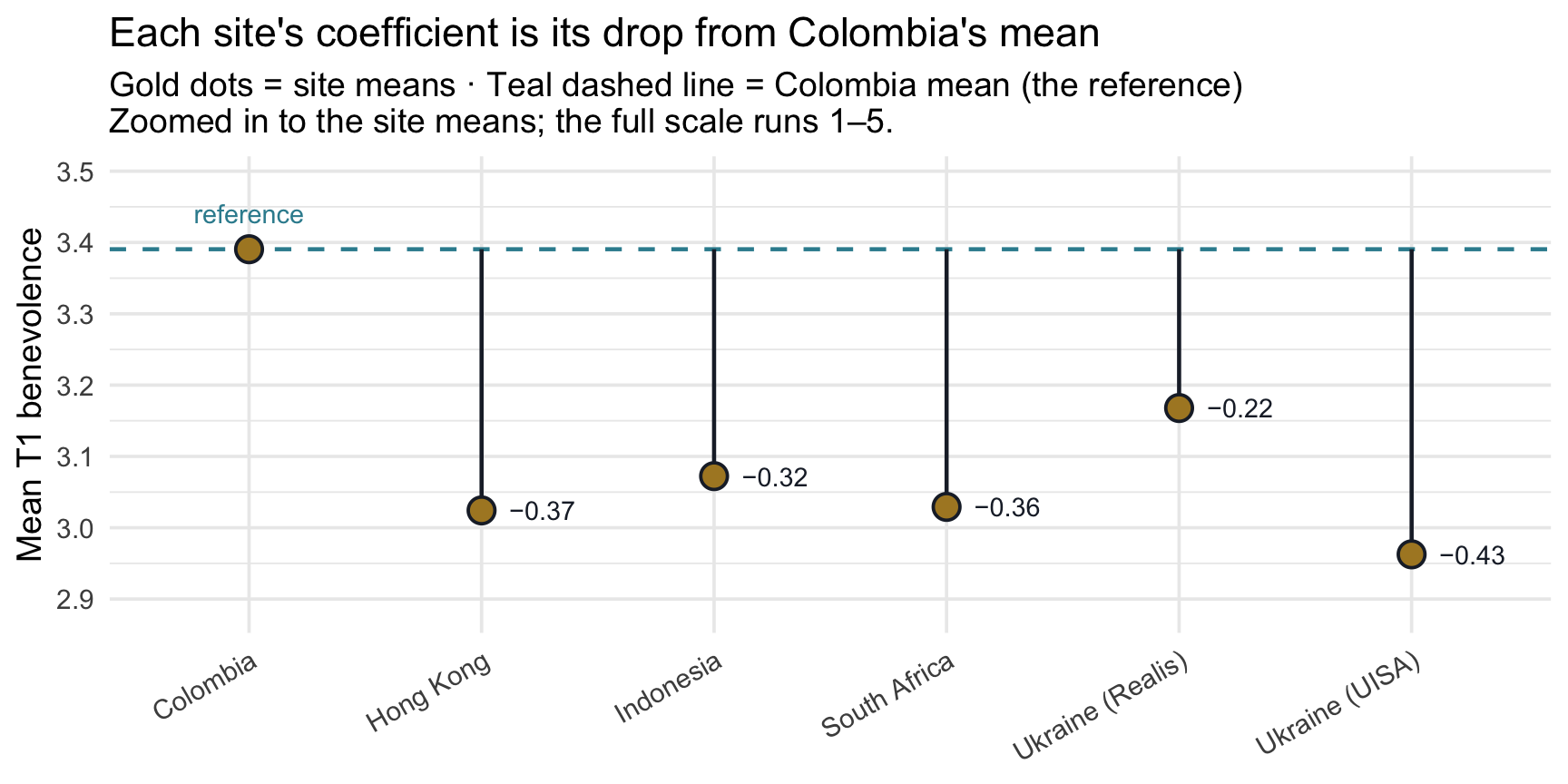
Read left to right: every other site’s gold dot sits below the teal Colombia line, with Ukraine (UISA) the lowest. The vertical gap between the line and each gold dot is that site’s regression coefficient — the same numbers tidy() reported above. The y-axis is zoomed in so the gaps are visible; on the full 1–5 scale they are small.
Inference for each contrast: the slope recipe, five times
Every row of the tidy() output above carries the same inference columns you met for the single slope in Part 1 — std.error, statistic, p.value, conf.low, and conf.high — and each one is built exactly the same way. Nothing new is needed; the recipe simply runs once per row:
- The critical value is \(t^*\) =
qt(p = 0.975, df), where df is the model’s residual degrees of freedom. - The 95% CI is \(b \pm t^* \cdot SE(b)\).
- The test statistic is the estimate divided by its standard error: \(t_\text{obs} = b / SE(b)\).
- The two-sided p-value is
2 * pt(q = abs(t_obs), df, lower.tail = FALSE).
Each row hands you an estimate and a standard error; those two numbers and the df generate everything else.
Here is that recipe computed by hand for the five site contrasts:
site_df     <- site_mod |> glance() |> pull(df.residual)   # n minus the 6 estimated coefficients
t_star_site <- qt(p = 0.975, df = site_df)                 # one critical value for every row

site_by_hand <- site_mod |>
  tidy(conf.int = TRUE) |>
  filter(term != "(Intercept)") |>
  mutate(
    ci_low  = estimate - t_star_site * std.error,
    ci_high = estimate + t_star_site * std.error,
    t_obs   = estimate / std.error,
    p_value = 2 * pt(q = abs(t_obs), df = site_df, lower.tail = FALSE)
  )

site_by_hand |>
  select(term, estimate, std.error, ci_low, ci_high, t_obs, p_value)
Every number matches the conf.low, conf.high, statistic, and p.value columns of tidy() exactly. Three things are worth noticing:
- One recipe, five times. Each row’s \(t_\text{obs}\) is that row’s estimate divided by that row’s standard error, just as for the single slope in Part 1. The smallest \(|t_\text{obs}|\) of the five is 4.54, for Ukraine (Realis).
- One \(t^*\) for every row. All five tests share the model’s residual degrees of freedom: n = 4,598 participants minus the 6 coefficients the model estimates (the intercept and five dummies), so df = 4,592 and \(t^*\) = 1.960. In general, the residual df is n minus the number of estimated coefficients, counting the intercept; M11 writes the same quantity as \(n - k - 1\), where k counts the slopes (the non-intercept coefficients: 5 here, one per dummy). That k is not the number of categories in the “\(k - 1\) dummies” rule above; same letter, different count. With this many df, \(t^*\) is essentially the Normal 1.96. In a small sample it is noticeably larger: with 15 df, for example, \(t^*\) = 2.13.
- One \(\sigma\), five different standard errors. The model uses a single residual SD, \(\sigma\) = 1.024, for every site. But each coefficient compares two group means, so its standard error is \(\sigma\sqrt{1/n_\text{Colombia} + 1/n_\text{site}}\): the fewer participants a site has, the larger its SE and the wider its interval. Hong Kong, the smallest site (n = 398), has the widest.
Each contrast with its 95% confidence interval
The figure below shows the same five coefficients on the difference scale, each with its 95% CI. The dashed line at 0 is “no difference from Colombia,” which is exactly the null hypothesis each row tests:
Show the code that built this figure
site_levels <- site_means |> pull(site) |> levels()   # Colombia first

site_by_hand |>
  mutate(site = sub("^site", "", term),
         site = factor(site, levels = site_levels[-1])) |>
  ggplot(aes(x = site, y = estimate)) +
  geom_hline(yintercept = 0, color = "#348C9E",
             linetype = "dashed", linewidth = 0.8) +
  geom_errorbar(aes(ymin = conf.low, ymax = conf.high),
                width = 0.15, linewidth = 0.9, color = "#4E5EAA") +
  geom_point(shape = 21, size = 4.5, fill = "#4E5EAA", color = "#1C2433", stroke = 1) +
  # the label goes after the site layers, so the x-axis is already a set of sites
  annotate("text", x = 0.55, y = 0.015, hjust = 0, vjust = 0, size = 3.8,
           color = "#348C9E", label = "Colombia (the reference): a difference of 0") +
  scale_y_continuous(breaks = round(seq(-0.6, 0.1, by = 0.1), 1),
                     labels = function(x) sub("^-", "−", sprintf("%.1f", x))) +
  coord_cartesian(ylim = c((site_by_hand |> pull(conf.low) |> min()) - 0.05, 0.1)) +
  labs(
    x = NULL, y = "Site mean − Colombia mean",
    title = "Each site's difference from Colombia, with its 95% confidence interval",
    subtitle = "Dots = site coefficients · Error bars = 95% CIs · Dashed line = no difference from Colombia"
  ) +
  theme(axis.text.x = element_text(angle = 30, hjust = 1))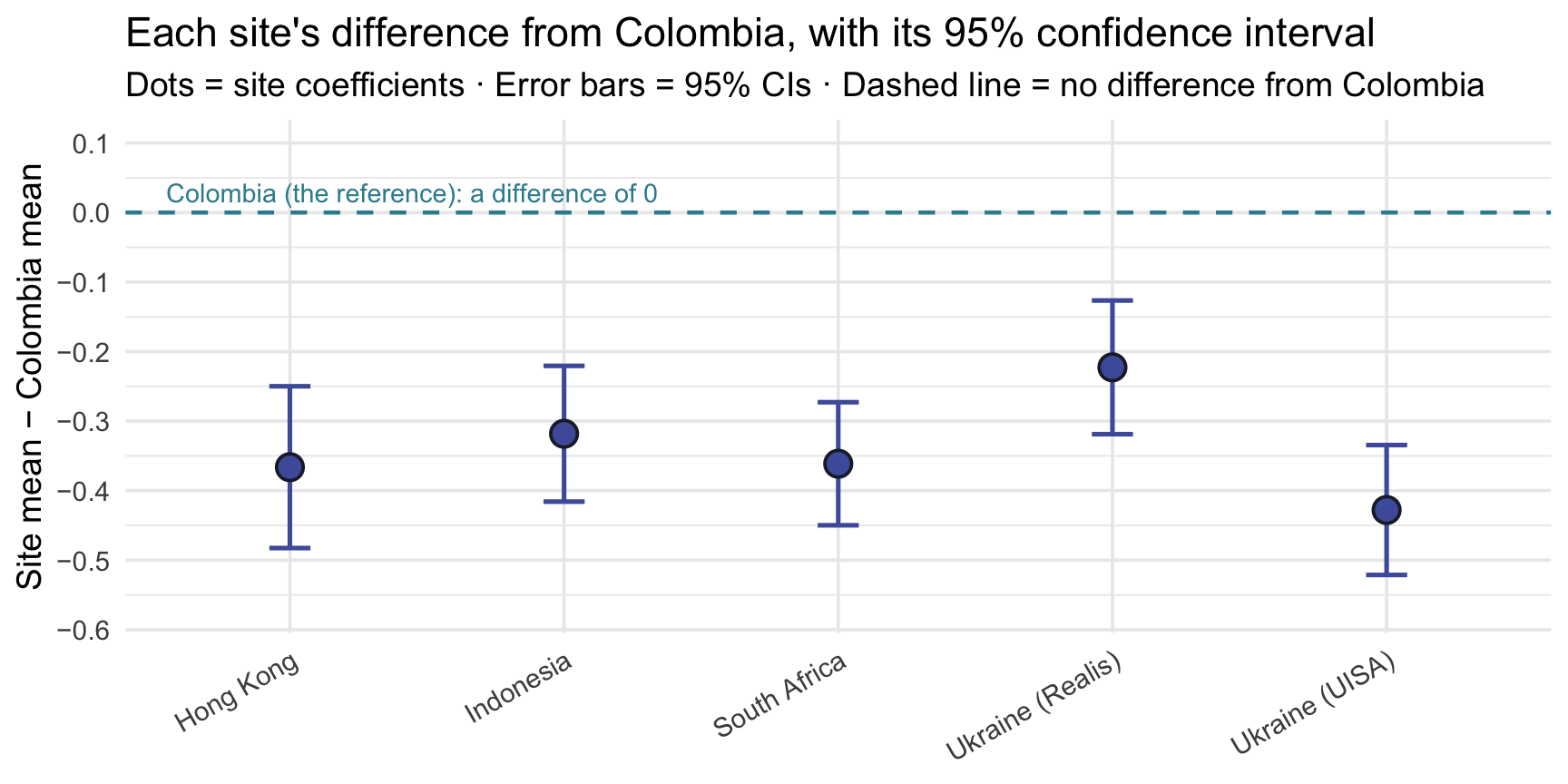
An interval that crossed the dashed line would be a contrast whose 95% CI includes 0, which in test terms means \(|t_\text{obs}| < t^*\) and p > .05. None crosses here. Even the smallest gap, for Ukraine (Realis), has an interval whose upper end is -0.127, still below 0. The intervals also differ in length, because the standard errors do (point 3 above).
Why draw the intervals on the difference scale? Because each interval describes a difference between two estimated means, and its standard error already carries the uncertainty in Colombia’s mean as well as the site’s. Drawing an interval around each site’s own mean and checking whether it reaches the Colombia line would be a different, and misleading, comparison.
Five contrasts and one omnibus test
The regression output answers two different kinds of question at once:
- Each coefficient row is its own test. The Hong Kong row tests whether Hong Kong’s population mean equals Colombia’s (\(H_0\): \(\beta_\text{HK} = 0\)), the Indonesia row tests the same thing for Indonesia, and so on: five rows, five separate tests, each with its own \(t_\text{obs}\), p-value, and CI.
- The F-statistic in glance() is a single joint test that all six site means are equal, or equivalently, that all five site coefficients are 0 at once. This is the omnibus test: F(5, 4592) = 22.49, the same F as M09’s one-way ANOVA (next section). A large omnibus F is evidence that the population site means are not all equal; it doesn’t say which differ.
These five comparisons are contrasts in exactly M09’s sense: each is a specific comparison between means. lm() gives you M09’s contrasts automatically: every group compared with the reference. When the reference is a natural baseline — a control condition, say — these are exactly the planned contrasts you would write down in advance. Here it isn’t (we chose Colombia only for convenience), so read them as descriptive comparisons. And because there are five of them, M09’s familywise caution applies: if all five null hypotheses were true, five tests at \(\alpha = .05\) would give more than a 5% chance of at least one false positive across the set.
These are contrasts to one reference, not a full pairwise comparison. Each site coefficient tests that site against the reference (Colombia) only — not every site against every other. If your goal is a complete site-by-site comparison, run every pairwise comparison with a multiplicity adjustment, exactly as in M09 Test 2: Tukey’s HSD, TukeyHSD(aov(t1_benevolence ~ site, data = reach)). Don’t read the reference contrasts as an all-pairs analysis.
Connection to the one-way ANOVA (M09 Test 2)
In M09 Test 2 we ran a one-way ANOVA on the Hofman boulder data — testing whether any of four groups had a different population mean. The procedure had a separate name (ANOVA), a separate statistic (F), and a separate output. And yet:
- The omnibus F from
lm(y ~ factor)is the same number the ANOVA reports. Both ask “is the variation between groups bigger than sampling variation alone would tend to produce if all the population means were equal?” - In this one-way ANOVA / regression setup, the model’s R² from glance() is the same as the ANOVA’s total \(\eta^2\): the proportion of the total variance explained by group membership. (You may later meet partial \(\eta^2\), which divides by a smaller total; in a one-way design the two are equal.)
- The intercept and slopes recover the group means in exactly the same way the ANOVA’s group-mean reporting does.
To make the connection literal, run a one-way ANOVA (using aov()):
aov(t1_benevolence ~ site, data = reach) |> tidy()Compare to glance()’s F-statistic, df, and p-value: identical. With the same outcome, the same grouping factor, and the same ordinary-least-squares, equal-variance model, a one-way ANOVA and lm(y ~ group) are two parameterizations of the same linear model, so the omnibus F, the degrees of freedom, and the p-value are identical: the “ANOVA test of site differences” and the “regression of benevolence on site” are the same procedure with a different name. The regression is more general because you can swap site for any other categorical variable, add a continuous covariate (M11), or build interactions (PSY 653) without ever leaving the lm() framework.
This is the regression-as-parent-framework point made concrete: M09’s two-sample t (Test 1) and one-way ANOVA (Test 2) are both special cases of lm(), and the unified syntax is just lm(outcome ~ predictor). (So is the paired t-test from the M09 bonus activity: it is the intercept-only case, lm(difference ~ 1).)
APA-style reporting
APA-style reporting · Simple Linear Regression (multi-category predictor)
Across 4,598 participants from six study sites, mean baseline benevolence differed across sites, F(5, 4592) = 22.49, p < .001, R² = .024. Compared with the reference site (Colombia, M = 3.39), each of the other five estimated site means was lower; the unadjusted reference contrasts were Hong Kong, b = -0.366, 95% CI [-0.483, -0.250]; Indonesia, b = -0.318, 95% CI [-0.416, -0.221]; South Africa, b = -0.361, 95% CI [-0.450, -0.273]; Ukraine (Realis), b = -0.223, 95% CI [-0.319, -0.127]; Ukraine (UISA), b = -0.428, 95% CI [-0.521, -0.334]. Site accounted for 2.4% of the variance in baseline benevolence (σ = 1.024).
One precision note: these contrasts and their CIs are unadjusted comparisons with the reference site (Colombia), not a full set of adjusted pairwise comparisons. If the research question were all pairwise site differences, the appropriate follow-up would be Tukey’s HSD, exactly as in M09 Test 2.
Note the structure: omnibus F with df → R² → reference-group mean (intercept) → each contrast with CI → \(\sigma\). When a categorical predictor has more than two levels, the omnibus F is the lead statistic; the individual coefficients are follow-up contrasts to the reference.
Looking ahead
You’ve now seen three uses of the same workflow:
| Module 10 example | Predictor type | What lm() returns | M09 connection |
|---|---|---|---|
| Part 1 — T2 ben ~ T1 ben (Hong Kong control) | Continuous | Intercept, slope, R², \(\sigma\) | (no direct M09 analog — new ground) |
| Part 2 — T2 ben ~ treat | Binary categorical | Intercept = Control mean; slope = Treatment − Control | Two-sample t-test (M09 Test 1) |
| Part 3 — T1 ben ~ site | Multi-category | Intercept = Colombia mean; five slopes = each site − Colombia | One-way ANOVA (M09 Test 2) |
Each example reused the same few pieces of code — lm(), tidy(), and glance(), plus augment() for fitted values and residuals — and the same four ingredients of inference (a coefficient, its SE, its CI, its p-value), exactly as introduced in M07–M09. What changed across examples was only the kind of predictor, and how to interpret the resulting coefficients.
One thing stayed constant across all three examples: the coefficient was the answer — a slope, a mean difference, or a contrast against a reference group, read straight off the tidy() table. In M11 that changes. Once a model holds several predictors at once, the coefficient table is no longer always the clearest answer to the research question. The better habit becomes: define the estimand first — the adjusted quantity the question actually asks for — and then query the fitted model to compute it. That shift from reading coefficients to computing estimands is the intellectual turning point of the regression arc, and it’s what M11 is built around.
Concretely: Module 11 (Multiple Linear Regression) asks what happens when you use more than one predictor at the same time — “Did the intervention raise follow-up benevolence, holding baseline benevolence constant?” Adjusting for baseline is a standard way to sharpen a trial’s treatment estimate (REACH ran it as a sensitivity analysis; the paper’s main model adjusted for site only), and a single-predictor model can’t do it. Module 12 (Model Assumptions) then checks that model — the diagnostic checks you run before trusting any regression’s coefficients or estimands. Fit → query → check, and then report with appropriate caution. (Whether the intervention works the same way for everyone — moderation / effect modification — is taken up in PSY 653.)
Summary
Core ideas: Simple Linear Regression
- Statistical models add a residual — unlike a deterministic relationship, a regression line says “outcome = what the model predicts + residual.” The residual is the part of each observation the fitted line doesn’t capture.
- The OLS line is the line of least squared residuals. Out of all possible lines, OLS picks the one whose residuals (when squared and summed) are smallest. Squaring keeps positive and negative misses from canceling; minimization defines “best fit.”
- Intercept and slope have plain-language meanings. \(b_0\) is the predicted \(y\) when \(x = 0\); \(b_1\) is the predicted difference in \(y\) between cases one unit apart on \(x\) — a comparison between people, not a change within a person. For categorical predictors, \(b_0\) becomes the reference-group mean and each \(b_k\) becomes a between-group mean difference.
- Two fit summaries. R² is the proportion of variance in \(Y\) explained — the variance-share story. \(\sigma\) is the typical scale of the residuals in raw outcome units — the typical-error story. The two are closely related, told in different units.
- For a continuous predictor, \(r^2 = R^2\), and the standardized regression slope equals the correlation \(r\). Different scalings of the same fitted line.
- Categorical predictors get dummy-coded. R creates \(k - 1\) dummies for \(k\) categories, with one level becoming the reference. The intercept is the reference-group mean; each dummy’s coefficient is its category’s mean − reference mean. Each coefficient is tested with the same recipe as a single slope (\(t_\text{obs}\) = estimate ÷ SE, one \(t^*\) from the residual df), and the omnibus F tests all of them at once.
- Two-sample t and one-way ANOVA are special cases of regression. The standard (Student’s) equal-variance two-sample t is
lm(y ~ binary_factor)— same numbers exactly. (Welch’s t-test relaxes equal variances and is closely related but not identical to the OLS default.) The one-way ANOVA islm(y ~ multi_category_factor), with the omnibus F identical between the two. This is the regression-as-parent-framework point — and Module 11 layers predictors on top.
Credits
- The reach_analysis data are a course-prepared subset of Ho, Worthington, Cowden, et al. (2024), International REACH forgiveness intervention: a multisite randomised controlled trial (BMJ Public Health).
- These Module materials draw on Gelman, Hill, & Vehtari’s excellent book Regression and Other Stories (2020, Cambridge University Press), which the authors make free to view for personal use from the book’s web page. It’s a strong next step for going deeper into Part 3’s regression material.
- Regression models are fit with base R’s lm(); tidy output uses broom (Robinson, Hayes, & Couch), effect sizes use effectsize (Ben-Shachar, Lüdecke, & Makowski), and the two-sample t comparison uses infer (Couch et al.).