Multiple Linear Regression

Learning Objectives

By the end of this Module, you should be able to:

The partial-effect core

• Build the conceptual chain from residualized gain to multiple linear regression — fit t2 ~ t1, inspect residuals by group, and show that the residual gap closely matches what an MLR with t2 ~ t1 + treat recovers automatically.
• Fit a multiple linear regression with lm(), mixing continuous and categorical predictors.
• Interpret slopes in the additive MLRs we fit as adjusted comparisons (partial effects) — the predicted difference in \(\hat{y}\) between people one unit apart on that predictor who share the same values of the other predictors.
• Center a continuous predictor and explain how centering reshapes the intercept’s interpretation in the multi-predictor setting.

Estimands, model comparison, and reporting

• State the quantity a research question asks us to estimate (the estimand), then report it from the fitted model with its uncertainty: here, the treatment coefficient and the adjusted means that predict() returns.
• Distinguish R² from adjusted R², and use ΔR² with a nested-model F-test (anova(m1, m2)) to ask whether a predictor (or set of predictors) adds information.
• Report MLR results in APA style, leading with the estimand of central interest and its CI, then the model’s F, R² / adjusted R², and the site block’s ΔR².

Structure and caveats

• Recognize that multisite data contain a grouping structure, and distinguish adjustment for between-site mean differences (including site as a categorical predictor) from methods that address residual dependence within site.
• Recognize the Table 2 fallacy — that control-variable coefficients in an adjusted model do not, in general, carry their own causal interpretation.
• Explain why adding a predictor can change a coefficient, and why adding baseline barely moves the treatment effect in a randomized trial.
• Explain when adjusting for baseline benevolence can be more precise than analyzing gain scores, and why a model should not adjust for variables measured after treatment.
• Explain the difference between a regression model used for prediction versus one used for causal inference, and the role of randomization in licensing causal language.

Overview

Where this fits — the Part 3 regression arc

Part 2 gave you a separate test for each design: a t-test for two groups, an ANOVA for several, a chi-square for a table of counts. Part 3 trades that toolbox for one tool, the linear regression model: an equation for how the average outcome changes with one or more predictors. It is also the foundation for most of the advanced models you’ll meet later in your training, from logistic and multilevel regression to structural equation models, so the ideas built in Part 3 carry forward into every one of them. The two-sample t and the one-way ANOVA from M09 turn out to be special cases of it, and the same model grows to hold several predictors at once, which is how researchers account for where people started and for other differences between them.

With a model as the tool, the work follows three steps. Modules 10–12 take one each, all on the REACH forgiveness trial you met in the Part 2 lectures:

• M10 · Fit — what relationship does the model estimate? (slopes, intercepts, residuals, fit)
• M11 · Query — what adjusted estimand answers the research question? (partial effects, adjusted comparisons) · ← you are here
• M12 · Check — are the model’s assumptions good enough to trust the inference? (diagnostics, remediation)

Underneath those three steps sits one habit that comes first: define the target — the quantity that would answer your research question — and then fit a suitable model, query it for the estimate, and check that the result is trustworthy enough to report. The same workflow carries into those more advanced models; only the model changes.

You finished M10 with a main result: participants assigned to the REACH workbook scored about half a point higher on follow-up benevolence. Because REACH was randomized, that gap has a causal basis — with one caveat about missing follow-ups that we’ll return to later. Then the reviewer’s email lands — “But did you adjust for where people started? For the site they were in? Is that half-point still there once you hold those constant?” Those are the questions that decide whether a finding survives review, and none of them can be answered well with a single predictor. Multiple linear regression is how you answer them.

M10 fit three one-predictor models, one per kind of predictor — continuous, binary, and multi-category (a single-factor linear model). Each model had one predictor on the right side of the formula. That’s a strong starting point, but it’s not the whole world. Real research questions almost always involve more than one predictor at a time, and the answer to “what does X do?” usually depends on what other variables are in the model alongside X.

Module 11 extends regression to handle two or more predictors simultaneously. The new framework is multiple linear regression (MLR), and the equation generalizes from M10’s single-predictor form

\[\hat{y}_i \;=\; b_0 \;+\; b_1 x_i\]

to the multi-predictor form

\[\hat{y}_i \;=\; b_0 \;+\; b_1 x_{1i} \;+\; b_2 x_{2i} \;+\; \cdots \;+\; b_k x_{ki}\]

where each \(x_j\) is its own predictor and each \(b_j\) is its own slope. For the additive models we fit here, each slope is a partial effect: \(b_j\) is the predicted difference in \(y\) between two people one unit apart on \(x_j\) who have the same values on all the other predictors. That idea — “holding all other predictors constant” — is the conceptual heart of MLR.

Starting from the question

This Module also adds a habit to how we read a fitted regression. M10 interpreted each coefficient directly, and for small models that works well. As models grow, it helps to start one step earlier: name the quantity the research question asks for (the estimand), then get it from the model. In REACH that quantity is the treatment contrast: how much higher T2 benevolence is under Treatment than under Control for comparable participants. In the additive models of this Module it equals a single coefficient, and the adjusted means come from predict(), the function you used in M10. Starting from the estimand also guards against the Table 2 fallacy we’ll meet later: reading every control-variable coefficient as a finding of its own.

One more distinction runs through M11: the same lm() can do two different jobs. In this Module’s REACH analyses, the job is to estimate one quantity the research question names: the treatment contrast. In the M11 lab, the job is to build a model that predicts an outcome, presidential vote shares. The tools are the same; what you report, and what can go wrong, differ. Part 6 sets the two side by side.

What we’ll do, in order

We’ll fit two MLRs on the REACH data, building up cumulatively:

1. Residualized gain — fit t2_benevolence ~ t1_benevolence (M10’s baseline-only model, refit on the complete-case analysis sample across both arms and all six sites), inspect residuals by treatment, and discover the MLR treatment coefficient from the picture. This is the conceptual on-ramp.
2. The baseline-and-treatment model — t2_benevolence ~ t1_benevolence.c + treat. The proper two-predictor MLR: the partial-effect interpretation, centering, inference for each coefficient, the precision gain, and R² and adjusted R².
3. From coefficients to estimands — name the adjusted treatment effect as a quantity, read it from the model, and get the two adjusted means with predict().
4. Adding site — t2_benevolence ~ t1_benevolence.c + treat + site. Adds the multi-category site predictor — the trial’s randomization stratum — to absorb between-site mean differences. We’ll see why some coefficients move when a predictor enters and others don’t, measure what site adds with ΔR² and a nested-model F-test, and dig into the Table 2 fallacy.
5. The treatment estimate from the model with site — predict for one site, then for every site, and see why the Treatment − Control gap is the same everywhere, so the estimate is the treatment coefficient. (It is an assignment-based, complete-case treatment contrast: everyone is analyzed in the arm they were assigned to, but only participants with a T2 score are included, so it is not the full-sample intention-to-treat analysis the published paper used.)

A closing Part takes up the two jobs of regression, the prediction-vs-causation distinction (an RCT licenses causal claims that an observational study would not), a warning about adjusting for post-treatment variables, and brief model-building principles.

What to master

Core — reading each coefficient as an adjusted comparison; residualized gain as the on-ramp; why adjusting for baseline benevolence sharpens a randomized comparison without changing what it estimates; centering; inference for each coefficient; R², adjusted R², ΔR², and the nested-model F-test; categorical predictors and the site block; why a coefficient can change when a predictor is added; the Table 2 fallacy; and the estimand-first report (define the target → fit → get the estimate from the model). The indigo boxes add context (how the dataset was built, missing data, fixed versus random effects); you don’t need them to use MLR well.

Packages used in this module

library(tidyverse)
library(here)
library(broom)
library(gtsummary)

Meet the data

This Module continues on the REACH Forgiveness intervention study (Ho et al., 2024; PDF) we met in M10.

The REACH study, in brief

REACH is the multisite randomized waitlist-controlled forgiveness-workbook trial from M10 — see M10’s Meet the data section for the full study, the REACH acronym, and the TRIM-18 measure. The four facts M11 leans on:

• Design. N = 4,598 adults across six sites, randomly assigned within site to receive the 2–3 hour workbook immediately (treat = Treatment) or after a 2-week delay (Control).
• Outcome. t2_benevolence — the benevolence subscale (higher = more forgiving) at the 2-week follow-up.
• Covariates M11 adds. t1_benevolence (baseline benevolence, also used centered as t1_benevolence.c) and site (the six-level randomization stratum).
• Focal question. Does the workbook raise follow-up benevolence — adjusting for where each participant started and which site they came from?

The full variable dictionary and codebook live in M10 and on the datasets & codebooks page.

Want to see how this dataset was built?

The cleaning, demographic re-coding, TRIM-18 reverse-coding, subscale construction, and reliability checks all live in a public Posit Cloud project: psy652-reach-data-prep. Open it any time you want to see the data-processing layer that comes before the analyses we run in this Module.

Loading and preparing the analysis sample

We load the data, build the centered baseline-benevolence predictor t1_benevolence.c, and perform complete-case analysis for the outcome, baseline benevolence, treatment, and site. All the REACH models below use these same rows:

reach <- read_rds(here("data", "reach_analysis.Rds"))

analysis <-
  reach |>
  drop_na(
    t2_benevolence,
    t1_benevolence,
    treat,
    site
  ) |>
  mutate(
    treat = fct_relevel(treat, "Control"),
    site = fct_relevel(site, "Colombia"),
    t1_benevolence.c = t1_benevolence - mean(t1_benevolence)
  )

analysis |>
  select(uid, site, treat, t1_benevolence, t1_benevolence.c, t2_benevolence) |>
  glimpse()

Rows: 3,965
Columns: 6
$ uid              <int> 1, 2, 3, 4, 5, 6, 7, 8, 9, 10, 11, 12, 13, 14, 15, 16…
$ site             <fct> Hong Kong, Hong Kong, Hong Kong, Hong Kong, Hong Kong…
$ treat            <fct> Control, Treatment, Treatment, Treatment, Treatment, …
$ t1_benevolence   <dbl> 2.666667, 3.666667, 4.333333, 4.000000, 3.000000, 2.3…
$ t1_benevolence.c <dbl> -0.48537201, 0.51462799, 1.18129466, 0.84796133, -0.1…
$ t2_benevolence   <dbl> 2.833333, 3.000000, 5.000000, 4.000000, 3.666667, 2.3…

A reminder on listwise deletion. Throughout PSY 652 we handle missing data with drop_na() — listwise deletion (or complete-case analysis). It’s the simplest approach, and it’s the one M05 (Describing Data with R) explains in full — with M10 adding the trial-specific differential-attrition angle this Module inherits. The short version: listwise deletion always costs information and precision, and it can also be biased when whether a participant has a follow-up score is related to the outcome in ways the analysis doesn’t account for — e.g., if the participants most likely to skip the 2-week follow-up differ on the outcome, the surviving sample becomes a biased view of the population, and so does the treatment-effect estimate. Data missing completely at random (MCAR) protect against that bias, but MCAR is one simple condition that does so, not the only one. More advanced courses develop the principled missing-data toolkit (multiple imputation via the mice package, FIML for SEM, the MCAR/MAR/MNAR taxonomy from Rubin, 1976). For M11, listwise deletion is the placeholder — sufficient for first exposure, not the destination.

The new piece of data prep is the centered baseline benevolence, t1_benevolence.c = t1_benevolence − mean(t1_benevolence). That’s the same recipe from M10’s Centering section; Part 2 leans on it so the intercept lands at an interpretable in-data value. The analysis sample has n = 3,965 participants (2,057 Control, 1,908 Treatment).

---

Part 1 — Residualized gain: how a second predictor adds information

The cleanest way to gain intuition for multiple linear regression is to discover it accidentally — by fitting a one-predictor model, looking carefully at the residuals it leaves behind, and noticing that those residuals have a systematic pattern by some other variable we didn’t put in the model. When that happens, the second variable is information the simpler model has been throwing away. Bringing it into the regression alongside the first will improve the fit and — more importantly — change the interpretation of the original predictor. That’s the central conceptual leap of MLR, and it’s much easier to see in action than to follow as an abstract claim.

The first arc of this Module explores that idea in three steps. By the end of Part 1 you will have fit your first MLR — almost by accident — and discovered the model’s central interpretive trick on your own. We’ll then look back and name what just happened.

Step 1 — What does baseline benevolence predict?

Think back to the simple linear regression we worked through in M10 — the one fit to the Hong Kong control arm, with T2 benevolence on the y-axis and T1 benevolence on the x-axis. The main finding there was that follow-up benevolence is partially forecastable from baseline benevolence: people who started higher tended to end higher. The line summarized the typical T1-to-T2 relationship, and the spread of points around it captured everything the line couldn’t account for.

M11 picks up from exactly that point, with two adjustments. First, we’ll fit the same baseline-only model — t2_benevolence regressed on t1_benevolence alone — to the complete-case analysis sample across both arms and all six sites, not just the Hong Kong control arm. This puts us on the analytic footing for our first MLR, which we’ll fit at the end of this Part (Step 3) and refine in Part 2. Second, we’ll watch what the model fails to predict — its residuals — while keeping track of the treatment-versus-control distinction, because that distinction is the second variable we’re eventually going to bring into the regression.

The baseline-only model has the familiar simple-linear-regression form (T2 is an abbreviation for follow-up benevolence, and T1 is an abbreviation for baseline benevolence):

\[\widehat{\text{T2}}_i \;=\; b_0 \;+\; b_1 \cdot \text{T1}_i,\]

with \(b_0\) (the intercept) and \(b_1\) (the slope on baseline benevolence) the two quantities lm() will estimate from the data. We fit it the same way as in M10:

baseline_only <- lm(t2_benevolence ~ t1_benevolence, data = analysis)

baseline_only |> tidy(conf.int = TRUE)

baseline_only |> glance() |> select(r.squared, sigma)

The output tells a coherent story. Baseline benevolence is a strong predictor of follow-up benevolence — the estimated slope is \(b_1\) = 0.588 (participants one point apart in baseline benevolence are predicted to differ by about three-fifths of a point at T2), and the model accounts for about 33% of the variation in T2 benevolence on its own (R² = .332). The fitted equation,

\[\widehat{\text{T2}}_i \;=\; 1.596 \;+\; 0.588 \cdot \text{T1}_i,\]

is the model’s expectation for each participant: given any T1 score, this is what the model thinks the corresponding T2 score will be, with no other information used.

Now let’s actually look at what that line says about the data. The figure below plots every participant in the analysis sample as one point, with T1 on the x-axis and T2 on the y-axis, and overlays the OLS regression line in black. Each participant is also color-coded by their treatment assignment — teal for Control, heather purple for Treatment — but for now the colors are purely visual: the line is fit to all participants together, with no knowledge of which arm of the trial each person is in. The colors are there so that when we come back to look at the residuals in Step 2, the eye can already track who ended up in which condition.

analysis |>
  ggplot(aes(x = t1_benevolence, y = t2_benevolence, color = treat)) +
  geom_jitter(width = 0.05, height = 0.05, alpha = 0.18, size = 1.0) +
  geom_smooth(aes(group = 1), method = "lm", formula = y ~ x,
              se = FALSE, color = "#1C2433", linewidth = 1.1) +
  scale_color_manual(values = c("Control" = "#348C9E", "Treatment" = "#945297")) +
  scale_x_continuous(breaks = 1:5) +
  scale_y_continuous(breaks = 1:5) +
  labs(
    x = "T1 benevolence (1–5)",
    y = "T2 benevolence (1–5)",
    title = "Step 1: a baseline-only prediction line",
    subtitle = "The black line is the prediction from t2_benevolence ~ t1_benevolence, \nwith no treatment information.",
    color = "Condition"
  ) +
  theme(legend.position = "top")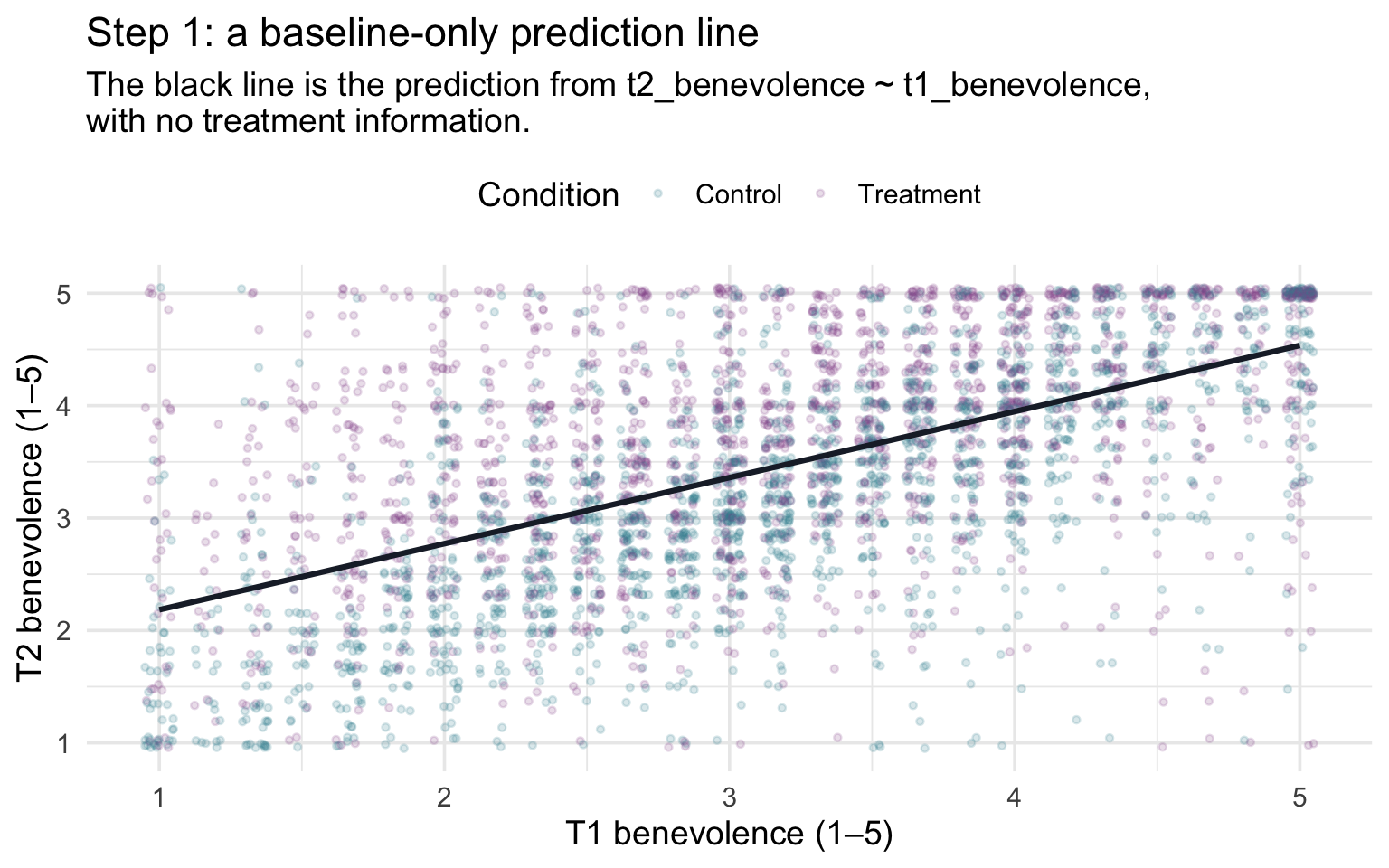

The black line is the model’s expectation for every participant — where each person’s T2 score should be, if the only piece of information we had about them was their baseline benevolence score. Some participants’ T2 scores land right on the best-fit line, others sit comfortably above it, and others below it. The vertical distance from each individual point down (or up) to the line is the participant’s residual — the gap between what actually happened and what the baseline-only model predicted. M10 introduced this quantity by name; here it earns a sharper interpretation. We’ll define the residual as the participant’s residualized gain: the portion of their follow-up benevolence that baseline benevolence alone cannot account for — the leftover signal the baseline-only model did not use. If an individual’s residual is positive, that means their T2 score is higher than we’d expect based on their T1 score. If an individual’s residual is negative, that means their T2 score is lower than we’d expect based on their T1 score.

Step 2 — Do the residuals differ by treatment?

Now comes the substantive question — and there’s a subtle pivot to make. In M10 we asked a simple, but crude, question:

“Did the treatment group end higher at T2 than the control group?”

Because REACH used random assignment, baseline benevolence is balanced between the two arms in expectation (on average, across all the ways the randomization could have come out) — Treatment and Control participants look statistically the same on every variable, measured or unmeasured, at the moment of enrollment. That balance is what protects the comparison from confounding. A confounder is a variable that affects both which group a person ends up in and their outcome (M01’s “third variable that drives both”); left alone, it can make the groups differ even when the treatment does nothing. Random assignment cuts that link, because a coin flip, not anything about the person, decides who gets the workbook. So a simple comparison of T2 means already estimates the workbook’s effect without bias by design (setting aside follow-up missingness, which Part 6 returns to); this is the M10 Part 2 model¹.

That, however, isn’t the most useful estimate. We’ve just seen that baseline benevolence is by far the strongest predictor of T2 benevolence we have — about a third of the variation in follow-up scores is forecastable from where each participant started. The simple “did the treatment group end higher?” comparison dumps all of that predictable structure into the residual error, leaving every individual’s variation around the group mean to count as unexplained noise. The result is a noisier answer than the data have to offer.

The sharper framing puts the baseline-only expectation into the picture. Instead of asking did the treatment group end higher at T2?, we ask: adjusting for where each person started, did the treatment arm score higher than the baseline-only model predicted — on average more than the control arm did? This is a question about gain beyond expectation — about residualized gain. The substantive content is the same (yes, the workbook arm scores higher); what changes is that we’ve stripped out the part of T2 that was already forecastable from T1 — leaving the comparison to the part of the outcome where a randomized treatment effect should show up most clearly. (Both comparisons estimate the same randomized effect; the adjusted one does so more precisely, as Part 2 shows.)

That question turns from rhetorical into computational the moment we have each participant’s residual sitting next to their treatment assignment in the same data frame. You know from M10 that broom::augment() computes those values for us — given a fitted model, it returns a new tibble with each participant’s predicted value (.fitted) and residual (.resid) attached to the original data:

resids <- baseline_only |>
  augment(data = analysis) |>
  select(treat, t1_benevolence, t2_benevolence, .fitted, .resid)

resids |> slice_head(n = 5)

For each participant in the resulting resids tibble, .fitted is the baseline-only model’s prediction (what M11 has been calling the expectation) and .resid is the gap between the participant’s observed T2 and that expectation. A positive residual means the participant ended above what the baseline-only model predicted for them; a negative residual means they ended below it.

The natural next step is to stop looking at residuals one participant at a time, and start looking at averages of residuals within each treatment arm. If the workbook is doing anything substantive, the average treatment-arm residual should sit clearly above the average control-arm residual — treated participants, as a group, should be exceeding their baseline-only expectations more than control participants do. Computing those averages takes one short pipeline:

mean_resid_by_treat <- resids |>
  group_by(treat) |>
  summarize(
    n = n(),
    M_resid = mean(.resid),
    SD_resid = sd(.resid)
  )

mean_resid_by_treat

# The gap between the two mean residuals (Treatment − Control)
resid_gap <- mean_resid_by_treat |> pull(M_resid) |> diff()

The pattern is the one the substantive theory predicts. Control participants have a mean residual of -0.242 — negative, which means that on average, given their T1 score, Control participants ended about a quarter point below what the baseline-only model expected. Treatment participants have a mean residual of 0.261 — positive and slightly larger in size, because the residuals sum to zero across both arms and the Treatment arm is the smaller of the two, so its mean residual has to be a little larger to balance. So Treatment participants averaged about a quarter of a benevolence point above their baseline-only expectation. The difference of those two means, 0.503, is the residualized treatment contrast. In words: on average, the treatment arm beat its baseline-only expectation by 0.503 of a benevolence point more than the control arm did.

The figure below makes the gap visible. Each dot is one participant’s residual; the black dots mark the two group means. Treatment-arm residuals (heather purple) center above zero and control-arm residuals (teal) center below it by about the same amount — the black mean dots make the shift visible — and the gap between those two mean dots is the residualized treatment contrast we just computed.

resids |>
  ggplot(aes(x = treat, y = .resid, color = treat)) +
  geom_jitter(width = 0.20, height = 0.0, alpha = 0.18, size = 1.0) +
  geom_hline(yintercept = 0, color = "#1C2433",
             linetype = "dashed", linewidth = 0.6) +
  stat_summary(fun = mean, geom = "point", shape = 21, size = 4.5,
               fill = "#1C2433", color = "#1C2433") +
  scale_color_manual(values = c("Control" = "#348C9E", "Treatment" = "#945297"),
                     guide = "none") +
  labs(
    x = NULL,
    y = "Residual (T2 observed − T2 predicted)",
    title = sprintf(
      "Step 2: do residualized gains differ by treatment? Difference = %.3f",
      resid_gap),
    subtitle = "Each dot is one participant's residualized gain. Black dots are group means."
  ) +
  theme(panel.grid.major.x = element_blank())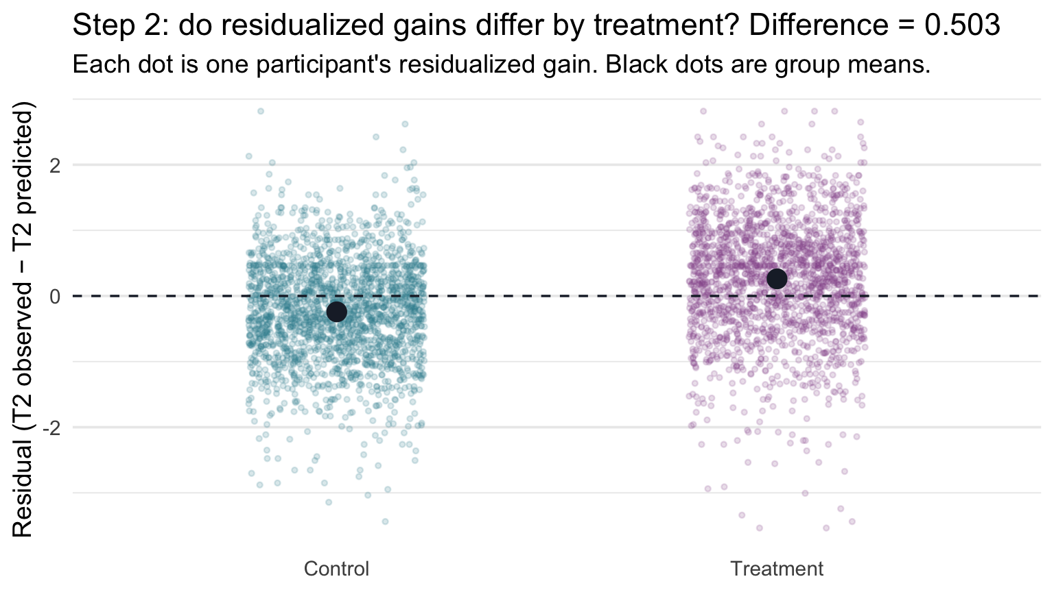

It’s worth pausing here for a second to register what just happened. We never fit a model that “knew” about treatment condition. The model we fit was the baseline-only model — T2 benevolence regressed on T1 benevolence alone, treatment nowhere in the formula. We then looked at the leftover variation the model couldn’t account for, broke that variation out by treatment arm, and noticed a clean shift between the two groups’ average residuals. That shift is the residualized treatment contrast — a close conceptual preview of the MLR treatment coefficient. Because treatment was randomized (so it’s nearly orthogonal to baseline benevolence), it lands very close to the proper one-step coefficient; the exact version residualizes both the outcome and treatment against baseline benevolence.

Step 3 — The MLR recovers the same number in one step

The two-step procedure we just walked through — fit, residualize, average by treatment — is conceptually clean and easy to follow. It’s also a slightly fragile way to do statistics in practice. The second step (taking the difference of mean residuals) doesn’t realize that the first step has already “used up” a degree of freedom estimating the slope on baseline benevolence, so the standard errors and p-values you’d get from a literal regression of .resid on treat would be slightly off. Acceptable for intuition-building; not what we’d actually report.

The fix is straightforward: do both steps inside a single regression that puts both predictors on the right-hand side of the formula at once. R’s lm() handles both, and the resulting model produces the right SEs and the right df without any extra effort on our part:

m1_uncen <- lm(t2_benevolence ~ t1_benevolence + treat, data = analysis)

m1_uncen |> tidy(conf.int = TRUE)

Look at the row for treatTreatment. The estimated coefficient is 0.503 — matching the difference of mean residuals (0.503) that we computed by hand at the end of Step 2, after rounding to three decimal places. The MLR barely changed the numerical answer from the simplified two-step procedure; it computed essentially the same residualized gain in one pass, with the right degrees of freedom built in.

We can verify the close agreement numerically by stacking the two answers side-by-side — the slope from a literal lm(.resid ~ treat) on the residual series, versus the treatTreatment coefficient from the proper two-predictor MLR:

two_step <- lm(.resid ~ treat, data = resids) |> tidy()
one_step <- m1_uncen |> tidy() |> filter(term == "treatTreatment")

bind_rows(
  two_step |> filter(term == "treatTreatment") |>
    mutate(approach = "two-step (lm(.resid ~ treat))") |>
    select(approach, estimate, std.error),
  one_step |> mutate(approach = "MLR (lm(t2 ~ t1 + treat))") |>
    select(approach, estimate, std.error)
)

The point estimates agree after rounding to three decimal places, and so do the standard errors — but they aren’t numerically identical: a small offset shows at the fourth decimal of the estimates (and the fifth decimal of the SEs). Two small things separate the two-step shortcut from the one-step MLR, both tiny at REACH scale but larger at small n. First, our shortcut residualizes only the outcome and leaves treat in raw form; the exact recipe residualizes both against baseline benevolence. Second, a literal lm(.resid ~ treat) uses n − 2 residual df rather than the correct n − 3. Both differences make the two-step SE very slightly too small. The one-step MLR avoids both issues automatically, which is why it’s the version we report.

What we’ve actually done

The model we fit in Step 3 was, formally, a multiple linear regression with two predictors — our first one. There are two complementary ways to understand what it does.

• The comparison view. lm(t2 ~ t1 + treat) compares Treatment and Control participants who have the same baseline benevolence. The treatment coefficient is the model’s predicted difference in T2 between those participants matched on baseline benevolence. This is the language Gelman, Hill, and Vehtari emphasize in Regression and Other Stories, and it’s the definition of the coefficient we’ll use from here on.
• The residual view. Baseline first predicts T2; treatment then asks whether those baseline-adjusted outcomes differ systematically between the two randomized arms. Our Step 2 residual comparison closely previews the treatment coefficient, and the match becomes exact when both the outcome and the treatment indicator are residualized against baseline benevolence.

These are two ways of understanding essentially the same adjusted comparison in this example. The first says what it means; the second makes the mechanics of “adjusting for baseline benevolence” visible. In REACH the answer is about half a benevolence point, and we recovered it two ways — once by hand (the difference of mean residuals in Step 2) and once with lm() (the treatment coefficient in Step 3).

Why not simply subtract the baseline benevolence score?

A simpler idea is the gain score: compute each person’s change, T2 − T1, and compare the two arms’ average gains. In a randomized trial that’s a legitimate analysis, but it quietly assumes that baseline benevolence carries forward one-for-one — a slope of exactly 1. Gelman, Hill, and Vehtari point out that analyzing gain scores “implicitly makes an unnecessary assumption, namely, that β = 1.” Here the estimated slope on baseline benevolence is about 0.59, well below 1, so the gain score subtracts more of baseline benevolence than the fitted relationship supports. Because treatment was randomized, using gain scores does not create systematic confounding by baseline benevolence: the gain-score treatment estimate (0.492) remains close to the adjusted regression estimate (0.503). But here the gain score is less precise: its SE is 0.029, compared with 0.026 for the regression, which estimates that slope instead of fixing it at 1. (If that slope really were 1, the two would be about equally precise; when it isn’t, the regression is the more precise.)

---

Part 2 — The baseline-and-treatment model: a properly fit two-predictor MLR

Part 1 was a discovery exercise: by examining the residuals of a baseline-only model, we closely approximated the MLR treatment coefficient by hand and then saw lm(t2_benevolence ~ t1_benevolence + treat) return the exact version of that number in one step. This Part takes that two-predictor MLR seriously — fits the centered version that we’ll use throughout the rest of the Module, walks through each coefficient as a partial effect, and names the precision gain that adding a strong covariate (a predictor included to account for differences among participants, rather than as the focus of the analysis) buys you.

Centering for an interpretable intercept

The uncentered model we discovered in Part 1 has a perfectly correct intercept — it just isn’t an interpretively useful one. In any multiple linear regression, the intercept \(b_0\) is the predicted value of the outcome when every predictor in the model equals zero simultaneously, with categorical predictors interpreted at their reference category. Here that means \(b_0\) is the predicted T2 benevolence for a Control participant (the treat dummy at 0) whose baseline benevolence is exactly zero. But the benevolence scale runs from 1 to 5; nobody can score zero on it. The intercept is therefore an extrapolation to a covariate profile that doesn’t exist in the data — a fine algebraic object but a poor anchor for understanding what the model predicts for a typical participant.

M10’s Centering: when zero isn’t a useful baseline section introduced the standard fix: subtract the predictor’s sample mean from each value before passing it to the model. In MLR the fix matters even more than in SLR, because once we have multiple predictors stacked together, the intercept becomes a compound summary — the predicted outcome when every continuous predictor sits at zero and every categorical predictor sits at its reference category. Each uncentered continuous predictor whose zero lies outside its observed range pushes the intercept further into extrapolation; centering it brings the intercept back to a value inside the data.

So we refit it with the centered baseline benevolence (t1_benevolence.c) we built in the Meet the data section above:

m1 <- lm(t2_benevolence ~ t1_benevolence.c + treat, data = analysis)

m1 |> tidy(conf.int = TRUE)

m1 |> glance()

Exactly as in M10’s centering example, the two slopes are unchanged by centering — the centered fit returns 0.585 for baseline benevolence and 0.503 for treat, identical to the uncentered fit from Part 1. Only the intercept moves, from a far-off-scale extrapolation to a meaningful in-data anchor.

Reading each coefficient as a partial effect

The fitted equation is

\[\widehat{\text{T2}}_i \;=\; \underbrace{3.207}_{b_0} \;+\; \underbrace{0.585}_{b_1} \cdot \text{T1.c}_i \;+\; \underbrace{0.503}_{b_2} \cdot \text{treat}_i\]

where \(\text{treat}_i = 1\) for Treatment-arm participants and \(0\) for Control-arm participants (the dummy coding R applied automatically when we passed the treat factor to lm(), with Control — the first level of the factor — as the reference category). Three coefficients to interpret:

• Intercept \(b_0\) = 3.207. The predicted T2 benevolence for the reference-profile participant — a Control-arm participant (\(\text{treat} = 0\)) at the average baseline benevolence (T1.c = 0, where T1.c is t1_benevolence.c in the equation above). The centered formulation does meaningful work here: with multiple predictors, the intercept becomes a clear summary of “the typical reference-condition participant” rather than the sum of several off-scale extrapolations.
• Baseline slope \(b_1\) = 0.585 (95% CI [0.560, 0.609]). Comparing two participants in the same arm whose baseline benevolence differs by one point, the model predicts the participant higher in baseline benevolence will score 0.585 points higher at T2.
• Treatment slope \(b_2\) = 0.503 (95% CI [0.452, 0.554]). The predicted difference in T2 benevolence going from Control to Treatment, holding baseline benevolence fixed — comparing two participants who started at the same T1 score.

These CIs, like every p-value and interval in this Module, are model-based: they rely on the regression assumptions that M12 checks, so treat them as provisional until then.

The “holding fixed” caveat on \(b_1\) and \(b_2\) is what makes each slope a partial effect: it’s the predicted difference in \(\hat{y}\) between people who differ on that one predictor and match on the others. Part 1’s residualized-gain demonstration is the operational meaning of that phrase — it’s what partialling out does to the model.

The partial-effect rule for any MLR coefficient

In a multiple linear regression with \(k\) slopes (one per predictor column; a categorical predictor with L levels contributes L − 1),

\[\hat{y}_i \;=\; b_0 \;+\; b_1 x_{1i} \;+\; b_2 x_{2i} \;+\; \cdots \;+\; b_k x_{ki},\]

each slope \(b_j\) is interpreted as a partial effect (in an additive model like the ones we fit in M11 — once a model includes interactions or nonlinear terms, some coefficients need more careful handling):

\(b_j\) is the predicted difference in the outcome between two cases that differ by one unit on \(x_j\) and have the same values on all the other predictors in the model.

That comparison is what “holding all other predictors constant” means in practice. It compares people; it doesn’t describe one person changing. Gelman, Hill, and Vehtari call a comparison “the safest interpretation of a regression”; reading \(b_j\) as what would happen if we raised someone’s \(x_j\) by one is a within-person, causal claim, and the data can’t support it on their own. A causal interpretation of the comparison needs design or identification assumptions; in REACH, random assignment supports an average causal interpretation of the Treatment–Control contrast, not a claim about any one person’s treatment effect. And a coefficient depends on what else is in the model: add or drop a predictor and the comparison changes, sometimes along with the number (Part 4 shows why).

Three closely related phrases describe this, each from a different angle: holding constant describes the comparison (people who match on the other predictors), adjusting for describes the fitted model (the other predictors are in it), and partialling out describes a computation (residualizing against the other predictors, as Part 1 did). The intercept \(b_0\) is the special case where all predictors equal zero simultaneously (continuous predictors at their zero value, categorical predictors at their reference category) — which reads as the reference-profile participant we met above when the continuous predictors are centered; leave them uncentered and zero is usually the off-scale extrapolation the centering discussion warned about.

Inference for each coefficient: the M10 recipe, unchanged

Every row of m1 |> tidy() carries the same inference columns as M10’s slopes, and they are built the same way. M10 Part 1 ran the recipe for one slope, and M10 Part 3 ran it once for each of five site contrasts; this model runs it once for each of its coefficients:

m1_df     <- m1 |> glance() |> pull(df.residual)   # n minus the 3 estimated coefficients
t_star_m1 <- qt(p = 0.975, df = m1_df)              # one critical value for every row

m1_by_hand <- m1 |>
  tidy(conf.int = TRUE) |>
  mutate(
    t_obs   = estimate / std.error,
    p_value = 2 * pt(q = abs(t_obs), df = m1_df, lower.tail = FALSE),
    ci_low  = estimate - t_star_m1 * std.error,
    ci_high = estimate + t_star_m1 * std.error
  )

m1_by_hand |>
  select(term, estimate, std.error, t_obs, p_value, ci_low, ci_high)

Every by-hand column matches tidy()’s statistic, p.value, conf.low, and conf.high exactly. Here is what carries over from M10 and what is new:

1. The recipe is identical. For every row, \(t_\text{obs}\) = estimate ÷ SE, \(t^*\) comes from the residual degrees of freedom, p = 2 * pt(q = abs(t_obs), df, lower.tail = FALSE), and the 95% CI is estimate ± \(t^* \cdot SE\).
2. The degrees of freedom count every coefficient. The model estimates three (the intercept, the slope on baseline benevolence, and the treatment slope), so df = n − 3 = 3,962 and \(t^*\) = 1.961. That’s M10’s rule, n minus the number of estimated coefficients counting the intercept, which MLR usually writes as \(n - k - 1\) with k = 2 slopes.
3. Each null hypothesis is now about a partial effect. The treatment row tests whether the treatment difference is 0 among participants with the same baseline benevolence; the baseline-benevolence row tests whether its slope is 0 within each arm. Each row is still its own separate test. (The intercept row tests whether the reference profile’s predicted T2 is 0, a value the 1–5 scale can’t take, so no one is asking that question.) The intercept’s confidence interval is a different matter. Because baseline benevolence is centered, its 95% CI, [3.172, 3.243], is the interval for the Control arm’s predicted mean T2 benevolence at average baseline benevolence, the same interval predict() returns for the Control profile in Part 3. In the uncentered model, the same row’s CI would describe a person with a baseline score of 0, whom the scale can’t produce.

And the omnibus test. As in M10, glance() reports one joint test: F(2, 3962) = 1260.9, p < .001, which tests whether both slopes are 0 at once — whether the model accounts for any of the variation in T2 at all. Its critical value is \(F^*\) = qf(p = 0.95, df1 = 2, df2 = df.residual(m1)) = 2.998; the F-test uses only the upper tail, so it puts all of \(\alpha\) = .05 there, unlike the two-sided t-tests. Our \(F_\text{obs}\) is far above it, and the model accounts for about 38.9% of the variation in T2 (R² = .389). In a model built to estimate one focal quantity, though, the omnibus F is rarely the question that matters. Here the question is the treatment row: an estimated difference of 0.503 points, 95% CI [0.452, 0.554].

The precision gain — adding a strong covariate

A natural follow-up question: now that we’ve adjusted for baseline benevolence, has the trial’s actual conclusion changed? Does adjusting tell us something different about the workbook than the simpler treat-only comparison would have? The answer turns out to be informative in two directions at once — the focal estimate stays where the trial’s design said it should stay, and the inference about that estimate gets sharper.

The cleanest way to see both effects is to fit the simplest possible RCT model — the one that uses only treatment as a predictor, with no adjustment for baseline benevolence at all — on the same participants, and lay the two models’ outputs side-by-side:

treat_only <- lm(t2_benevolence ~ treat, data = analysis)

treat_only |> tidy(conf.int = TRUE)

treat_only |> glance() |> select(r.squared, sigma)

Quantity	SLR lm(t2 ~ treat)	MLR lm(t2 ~ t1.c + treat)	What moved?
Treatment coefficient	0.519	0.503	negligible: -0.016
Treatment coefficient SE	0.0323	0.0261	shrinks by ~19%
\(\sigma\) (residual SD)	1.017	0.820	shrinks substantially
R²	.061	.389	jumps substantially

The point estimate of the treatment effect barely moves — which is what we’d expect under random assignment, because baseline benevolence is approximately balanced between the two arms and there’s nothing for the adjustment to “soak up” on the focal coefficient. But the standard error on the treatment coefficient drops by about 19%.

Why? In the treat-only model, a Control participant who started high (T1 = 5) tends to end high at T2, so contributes a large positive residual, \(y_i - \bar{y}_\text{Control}\); one who started at T1 = 2 tends to contribute a negative one. All that within-condition variation goes into \(\sigma\). In the MLR, the inclusion of the baseline benevolence score accounts for a good share of that within-condition variation — what remains in the residuals is much smaller. A smaller residual variance tends to improve coefficient precision. For the treatment coefficient here, baseline benevolence is nearly orthogonal to treatment because of randomization, so the reduction in residual noise dominates and its SE becomes substantially smaller.

This is the practical payoff of adding a strong covariate to an RCT: the focal effect’s magnitude barely changes, but its precision improves noticeably. One precise caveat: in expectation, randomization means covariate adjustment should not systematically move the treatment estimate — but in any one finite sample it can shift slightly, because randomization balances covariates only approximately. Regulatory guidance on trial analysis — the European Medicines Agency’s Guideline on adjustment for baseline covariates in clinical trials (2015) and the U.S. FDA’s Adjusting for Covariates in Randomized Clinical Trials for Drugs and Biological Products (2023) — recommends pre-specified adjustment for strong baseline covariates for exactly this reason. Gelman, Hill, and Vehtari make the same point: under a clean randomization, adjusting for a pre-treatment predictor “does not change what we are estimating”; it estimates the same treatment effect more precisely.

R² and adjusted R²

Our R² is .389, up from the treat-only model’s .061. The two predictors together account for about 38.9% of the variation in T2 benevolence — most of it accounted for by baseline benevolence, with a smaller incremental piece from treatment.

There’s a subtle problem with R² as a model-comparison tool, though: adding any predictor to a regression cannot decrease R², even if the predictor is pure noise. Random predictors have non-zero correlations with the outcome by chance, so they capture some tiny share of variance. As you add predictors, R² creeps up mechanically.

Adjusted R² corrects this by penalizing models that have more predictors:

\[R^2_{\text{adj}} \;=\; 1 - \frac{(1 - R^2)(n - 1)}{n - k - 1}\]

where \(k\) is the number of slopes (the non-intercept coefficients) and \(n\) the sample size. Here, adjusted R² is .389 — essentially identical to R², because n is huge (3,965) and the penalty for \(k = 2\) slopes is microscopic. Adjusted R² becomes especially useful when comparing models with different numbers of predictors, particularly at more modest sample sizes; we’ll lean on it in Part 4 when we add the multi-category site predictor.

R² never decreases when you add a predictor. Adjusted R² can — and should — decrease if you add a predictor that captures less variance than the penalty deducts. If adjusted R² rises, the predictor clears a low bar; if it stays flat or drops, it adds little. For a formal comparison, use the nested-model F-test (Part 4) when one model is nested in the other, or information criteria (AIC and BIC, which more advanced courses cover).

Two cautions about reading any R². First, a small R² is not a flaw: the treat-only model’s R² is only .061 even though the trial shows a clear effect. It’s small because most of the variation in T2 comes from where people started and from everything else in their lives. Second, R² depends on how spread out the predictors are in your sample; a study that recruited a narrower range of baseline benevolence scores would show a smaller R² even if the line and \(\sigma\) were the same.

---

Part 3 — From coefficients to estimands

The standard way to “report a regression” is to interpret each coefficient one by one, which is what Part 2 just did. That works for a two-predictor model, but it gets strained as models grow: with many categorical predictors, interactions, or curves, reading coefficients one at a time gives a fragmented picture and invites the Table 2 fallacy (Part 4). A sturdier habit, laid out clearly by Rohrer and Arel-Bundock (2026) (PDF), is to start from the question:

1. Define the target quantity (the estimand) the research question asks about. For example: “predicted T2 benevolence under Control at the mean baseline benevolence,” or “the predicted Treatment − Control difference for participants with the same baseline benevolence.”
2. Fit a model suited to that question and the design of the study.
3. Get the estimate from the model, with the right inputs and comparisons.
4. Report the estimate with its uncertainty. A coefficient is useful when it directly answers the question, but it need not be the centerpiece of every result.

The adjusted treatment effect

For the baseline-and-treatment model, the research question is:

Adjusting for baseline benevolence, how much higher is predicted T2 benevolence for a Treatment-arm participant than for a Control-arm participant with the same baseline benevolence?

In this additive model that estimand is the treatment coefficient: \(b_2\) = 0.503, 95% CI [0.452, 0.554]. Because the model has no interaction, the Treatment − Control gap is the same at every baseline value, so no further calculation is needed. That won’t stay true in richer models: once treatment interacts with another predictor, the gap can depend on where you look. That’s why the habit of naming the estimand first is worth building now, while every answer can be checked against tidy().

The two adjusted means

A paper would also report the two adjusted means: predicted T2 benevolence under each condition for participants at the same baseline benevolence. Here we pin baseline benevolence at its mean, which, because t1_benevolence.c is centered, is the value 0. These come from predict() with interval = "confidence", exactly as in M10: hand it a small tibble that describes the participants you want predictions for, one row per profile.

profiles <- tibble(
  treat = c("Control", "Treatment"),
  t1_benevolence.c = 0
)

adj_means_m1 <- profiles |>
  bind_cols(predict(m1, newdata = profiles, interval = "confidence", level = 0.95))

adj_means_m1

Notice that we simply write the label, "Control". You may remember from M10 that it’s safest to store a categorical predictor as a factor before fitting, so you control its levels and its reference group — but that advice is about fitting the model. Once m1 is fit, it remembers treat’s two categories, so predict() only needs to see the label. (Misspell it, and R stops with a clear error rather than guessing.)

Read the call from the inside out. predict() takes the fitted model and the newdata tibble, and interval = "confidence" asks for a confidence interval around each prediction (level = 0.95 sets its width). It returns three columns, one row per profile: fit, the prediction itself, and lwr and upr, the lower and upper ends of its 95% CI. bind_cols() then attaches those columns to profiles, so each prediction sits next to the profile it describes. Two adjusted means:

• Under Control, at mean baseline benevolence: 3.207. This is exactly the intercept \(b_0\), and its CI is the intercept row’s CI from tidy(): with centering, the intercept is the predicted outcome for the reference condition at T1.c = 0.
• Under Treatment, at mean baseline benevolence: 3.710, which is \(b_0 + b_2\) = 3.207 + 0.503.

Nothing here is new arithmetic. What changes is that the question and the answer are phrased in the same language — “adjusted mean T2 benevolence at average baseline benevolence, under condition X” — with each mean carrying its own CI.

Visualize the adjusted means

Plots of this shape — adjusted group means with their CIs — are the standard picture of an adjusted RCT analysis, and they put the question and its answer on the same graph.

Turning predict() output into a graph takes one idea: every column the graph needs is already in the tibble. Each row of adj_means_m1 is one profile. fit says where the dot goes, and lwr and upr say where its interval starts and stops. So in ggplot() we map x = treat, y = fit, ymin = lwr, and ymax = upr, and geom_pointrange() draws each dot and its interval in a single layer:

adj_means_m1 |>
  ggplot(aes(x = treat, y = fit, color = treat)) +
  geom_pointrange(aes(ymin = lwr, ymax = upr),     # dot at fit; line from lwr to upr
                  linewidth = 1.0, size = 0.5) +
  scale_color_manual(values = c("Control" = "#348C9E", "Treatment" = "#945297"),
                     guide = "none") +
  scale_y_continuous(limits = c(2.8, 3.9)) +
  labs(
    x = NULL,
    y = "Adjusted T2 benevolence",
    title = "Model-implied means by condition",
    subtitle = "Holding baseline benevolence at its sample mean; intervals are 95% CIs."
  ) +
  theme(panel.grid.major.x = element_blank())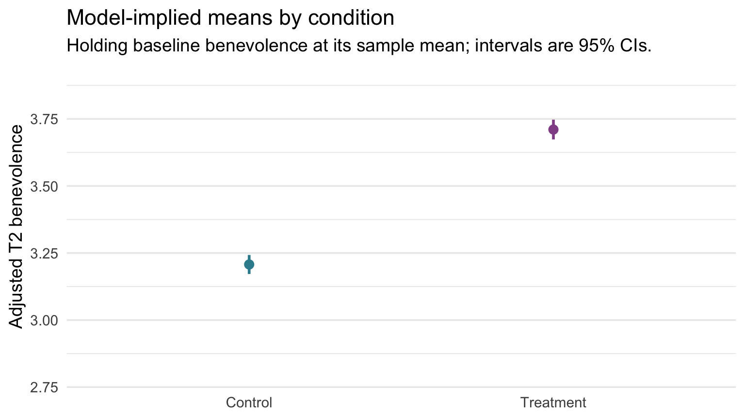

The vertical distance between the two dots is the adjusted treatment effect. One caution when reading it: don’t judge the Treatment − Control difference from whether the two intervals overlap. Each interval describes one adjusted mean; the interval for the difference itself is the treatment coefficient’s CI, [0.452, 0.554].

How do individual participants compare?

That graph answers the trial’s question, how much higher is the average?, and it answers it precisely. But notice what it leaves out: the participants. Its y-axis spans only about one benevolence point, and nothing in it shows how much individuals vary. Remember the boulder study from M09: Hofman, Goldstein, and Hullman (2020) found that readers shown only CIs were willing to pay more for the same effect than readers shown prediction intervals, because a narrow interval makes an effect look bigger than it is for any one person. So let’s draw the same result three more ways.

Version 1 — every participant, adjusted to the average baseline

To put participants on this graph, each one’s T2 score has to be adjusted the same way the means were. augment(), from Part 1, already has the piece we need: each participant’s residual, .resid, how far their T2 landed above or below the model’s prediction for them. A participant’s adjusted score is that residual placed around their arm’s adjusted mean:

\[\text{adjusted T2}_i \;=\; \text{adjusted mean for their arm} \;+\; \text{residual}_i\]

That works out to \(\text{T2}_i - b_1 \cdot \text{T1.c}_i\): the part of a participant’s T2 that the model credits to starting above or below the average is taken away. (For someone who started one point above average, that’s \(b_1\) = 0.585 points.)

adjusted_points <- m1 |>
  augment(data = analysis) |>                                       # adds .fitted and .resid
  left_join(adj_means_m1 |> select(treat, fit), by = "treat") |>    # each arm's adjusted mean
  mutate(adjusted_t2 = fit + .resid)

# Each arm's average adjusted score
adjusted_points |>
  group_by(treat) |>
  summarize(mean_adjusted_t2 = mean(adjusted_t2))

Each arm’s average adjusted score, 3.207 and 3.710, is exactly the adjusted mean predict() returned. (That isn’t luck: least squares makes the residuals average zero within each arm.) Some adjusted scores land outside the 1–5 scale, ranging from -0.08 to 6.26, because they are model-based scores, not observed ones.

The graph has two layers, and each layer brings its own data: the jittered points come from adjusted_points, one row per participant, and the black dots, one per arm at its adjusted mean, come from adj_means_m1, one row per profile.

ggplot() +
  # Layer 1: one point per participant
  geom_jitter(data = adjusted_points,
              aes(x = treat, y = adjusted_t2, color = treat),
              width = 0.20, height = 0, alpha = 0.15, size = 0.9) +
  # Layer 2: one dot per arm, at its adjusted mean
  geom_point(data = adj_means_m1,
             aes(x = treat, y = fit),
             color = "#1C2433", size = 3) +
  scale_color_manual(values = c("Control" = "#348C9E", "Treatment" = "#945297"),
                     guide = "none") +
  labs(
    x = NULL,
    y = "Adjusted T2 benevolence",
    title = "Individual participants and the adjusted means",
    subtitle = "Points: each participant's T2, adjusted to the average baseline.\nBlack dots: the adjusted means."
  ) +
  theme(panel.grid.major.x = element_blank())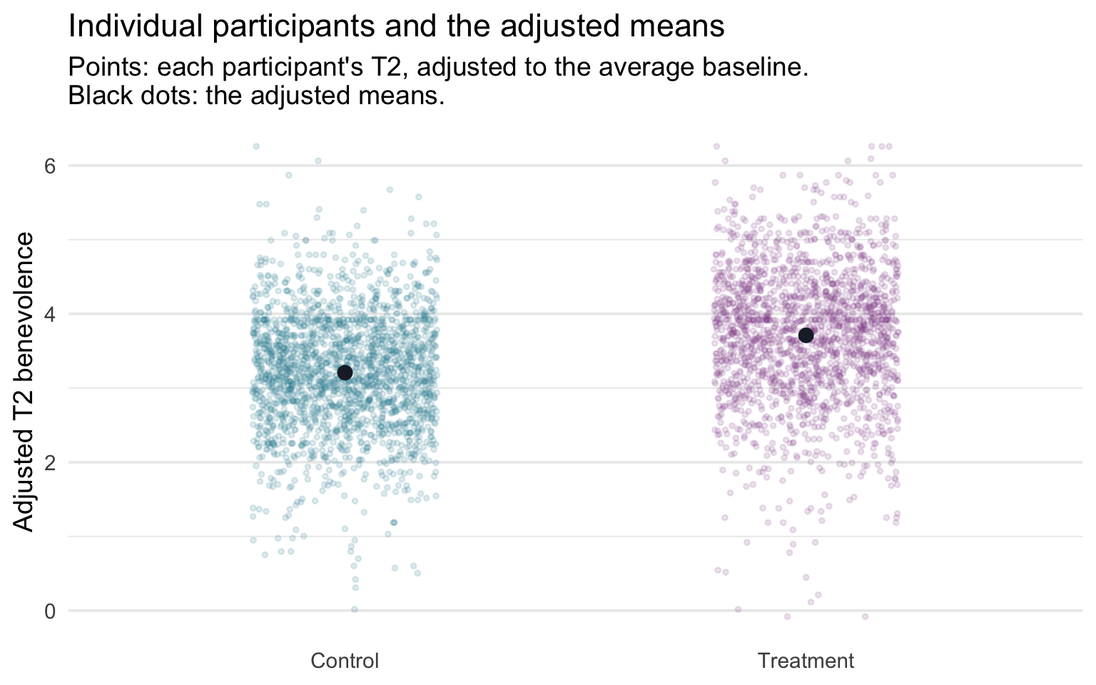

We left the CIs off this graph: at about 0.07 of a point wide, they would hide behind the black dots. The participants, meanwhile, spread across several points and overlap heavily between the arms. Both are true at once: the average difference is estimated precisely, and individuals vary a great deal around their arm’s average.

Version 2 — the prediction interval

The second version swaps the cloud of points for a prediction interval (PI): the range that should cover the T2 score of one new participant at the average baseline, in each arm. It comes from the same predict() call with one argument changed, exactly as in M10:

pred_int_m1 <- profiles |>
  bind_cols(predict(m1, newdata = profiles, interval = "prediction", level = 0.95))

pred_int_m1

The fit column is unchanged: the best prediction for a new participant is the same adjusted mean. Only lwr and upr move, and they move a lot. The PI is about 3.22 points wide, roughly 45 times the CI’s width, because it adds the person-to-person scatter (\(\sigma\) = 0.82) to the uncertainty about the mean. Descriptively, about 95% of the participants’ adjusted scores happen to fall inside their arm’s PI, consistent with the size of the model’s residual scatter. The PI’s formal 95% describes something else: across repeated samples, how often an interval built this way covers a new participant’s score.

To draw it, map the columns the same way as before: a wide, pale geom_linerange() from ymin = lwr to ymax = upr for each PI, and a geom_point() at y = fit for the predicted score. (As in Version 1, the CIs would hide behind the dots, so we leave them off.)

pred_int_m1 |>
  ggplot(aes(x = treat, color = treat)) +
  geom_linerange(aes(ymin = lwr, ymax = upr),        # the 95% PI: a wide, pale bar
                 linewidth = 8, alpha = 0.25) +
  geom_point(aes(y = fit), size = 3) +               # the predicted score
  geom_hline(yintercept = 5, linetype = "dashed", color = "grey50") +
  scale_color_manual(values = c("Control" = "#348C9E", "Treatment" = "#945297"),
                     guide = "none") +
  labs(
    x = NULL,
    y = "Predicted T2 benevolence",
    title = "Where one new participant's score might land",
    subtitle = "Bars: 95% prediction intervals at the average baseline. Dots: the predicted score.\nDashed line: the top of the 1–5 scale."
  ) +
  theme(panel.grid.major.x = element_blank())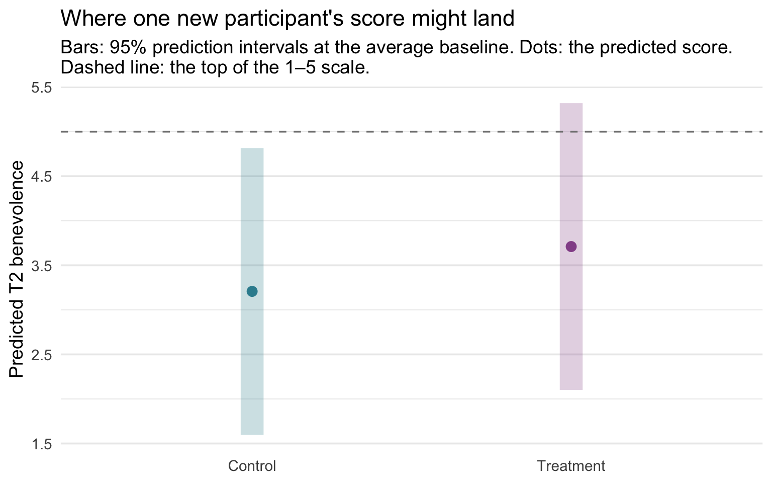

Set this graph beside the CI graph above and read the two intervals as answers to two different questions. The CI answers the trial’s question: where is each arm’s average at the same baseline benevolence? Those CIs were about 0.07 of a point wide, so the difference in averages is estimated precisely. The PI answers a question about one person: where will a new participant’s T2 land? The two PIs overlap almost entirely, so knowing someone’s arm tells you much less about their own score than the CIs alone suggest. Report the interval that matches the question you’re answering, and when the audience might read an average as a promise about individuals, show both. (The Treatment PI’s upper end, 5.32, passes 5, the top of the scale. The PI assumes Normal scatter around the prediction, and scores piled near a ceiling don’t quite behave that way, which is one of the checks M12 makes.)

Version 3 — both intervals on one scale

Each graph so far shows at most one kind of interval. To see the CI and the PI together, draw them on the same y-axis as bars of the same width, and leave off the dots that were hiding the CIs. Both layers use the same mapping, ymin = lwr and ymax = upr: the pale bars come from pred_int_m1 and the dark bars from adj_means_m1.

ggplot() +
  # Layer 1: the 95% PIs (tall, pale)
  geom_linerange(data = pred_int_m1,
                 aes(x = treat, ymin = lwr, ymax = upr, color = treat),
                 linewidth = 8, alpha = 0.25) +
  # Layer 2: the 95% CIs (short, dark), drawn at the same width
  geom_linerange(data = adj_means_m1,
                 aes(x = treat, ymin = lwr, ymax = upr, color = treat),
                 linewidth = 8) +
  scale_color_manual(values = c("Control" = "#348C9E", "Treatment" = "#945297"),
                     guide = "none") +
  labs(
    x = NULL,
    y = "Predicted T2 benevolence",
    title = "The CI and the PI on one scale",
    subtitle = "Tall pale bars: 95% PIs for one new participant.\nShort dark bars: 95% CIs for the adjusted means."
  ) +
  theme(panel.grid.major.x = element_blank())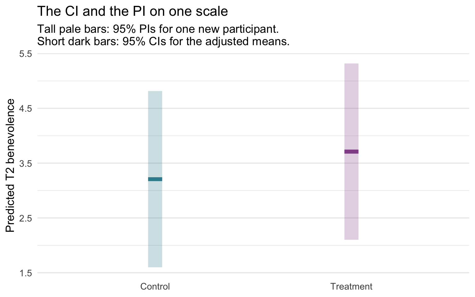

Both intervals are centered on the same adjusted mean; only their heights differ. The dark CI is a sliver, about 0.07 of a point, inside a PI about 3.22 points tall. That contrast is the lesson in one picture, and it’s why the two stay on one axis: putting them in separate side-by-side panels would need two different y-axes, and the difference in size would disappear.

---

Part 4 — Adding site: a multi-category predictor

Why include site?

You might reasonably push back here: Part 1 argued that the unadjusted comparison is already unbiased, so why add five more coefficients? REACH randomized participants within each site, so treatment is balanced across sites by design, and site is not a confounder. (Our complete-case analysis adds a separate caution: dropping participants without a T2 score can weaken that balance, whether or not site is in the model.) We add site anyway because it is the trial’s randomization stratum and a source of systematic between-site differences: participants at the same site share recruitment channels, cultural context, language of administration, and local conditions during data collection.

Including site as a categorical predictor fits a separate intercept per site (M10 Part 3’s dummy coding), absorbing those between-site mean differences. That buys a very small precision gain (site predicts the outcome and, by design, is nearly unrelated to treatment) and a site-adjusted estimand that respects the blocking structure. It is also what the REACH investigators did: their preregistered primary analysis regressed each T2 outcome on treatment group with fixed effects of site (Ho et al., 2024). Gelman, Hill, and Vehtari give the same advice for blocked experiments, recommending the blocking variables “both for concerns of bias and efficiency.” What site indicators do not do is guarantee independent residuals within a site; cluster-robust standard errors and multilevel models are the fuller tools for that (see the box below).

Fixed effects vs random effects. Including site as a categorical predictor treats each site’s intercept as a fixed effect: estimated separately, with no pooling toward an overall mean. A multilevel (mixed-effects) model instead treats site effects as arising from a common distribution and partially pools them toward the grand mean, which helps when there are many groups, when the between-site variation is itself of interest, or when generalizing beyond the observed sites is part of the target. With only six sites that also served as randomization strata, fixed indicators are the simple, transparent choice here (and with so few sites, cluster-robust standard errors are themselves limited). Multilevel models are covered in PSY 653.

Showing the between-site differences

Before fitting the model with site, it’s worth stopping to look at the data the new predictor will absorb. The visible pattern in the raw data is that average T2 benevolence differs across sites, in addition to differences between treatment arms. (Whether residuals remain correlated within a site after accounting for those site means is a separate question, one a picture of means can’t settle.) If we plot follow-up benevolence by site, with the two treatment arms overlaid, we should see two things at once: a visible site-to-site shift in the cloud heights (the between-site mean differences site will absorb), and the observed Treatment–Control difference within each site. The common treatment difference we later draw from the additive regression is a model assumption, not something the raw plot itself guarantees.

analysis |>
  ggplot(aes(x = site, y = t2_benevolence, fill = treat)) +
  geom_violin(position = position_dodge(width = 0.85),
              alpha = 0.30, color = NA, width = 0.8) +
  geom_boxplot(position = position_dodge(width = 0.85),
               width = 0.18, fill = "white", outlier.alpha = 0.20) +
  stat_summary(aes(group = treat), fun = mean, geom = "point",
               position = position_dodge(width = 0.85),
               shape = 21, size = 3, fill = "#AD872B", color = "#AD872B") +
  scale_fill_manual(values = c("Control" = "#348C9E", "Treatment" = "#945297")) +
  scale_y_continuous(breaks = 1:5) +
  labs(
    x = NULL, y = "T2 benevolence (1–5)", fill = "Condition",
    title = "T2 benevolence by site and condition",
    subtitle = "Gold dots = group means. Within each site, the treatment mean is higher than the control mean."
  ) +
  theme(axis.text.x = element_text(angle = 30, hjust = 1),
        legend.position = "top",
        panel.grid.major.x = element_blank())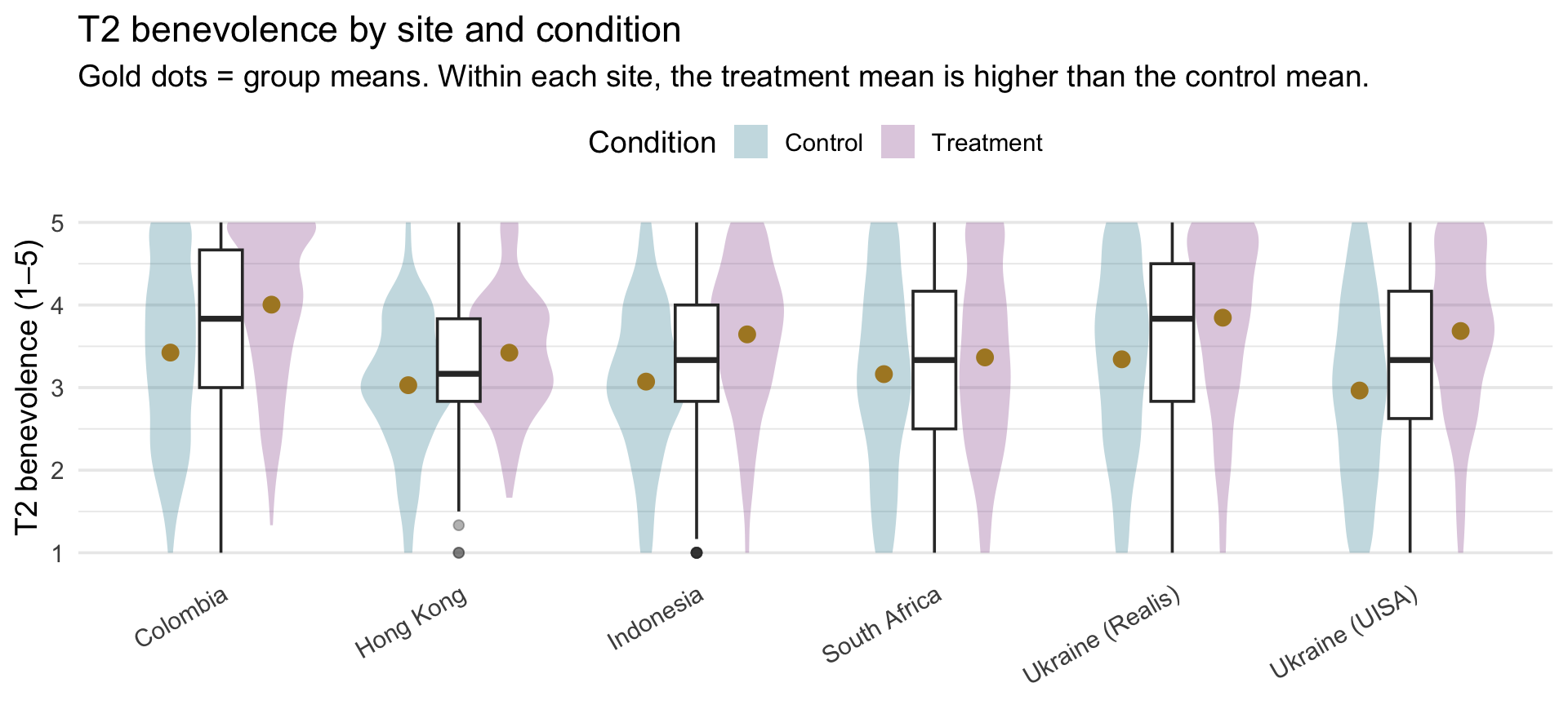

Two patterns to notice:

1. Within each site, treatment sits above control in this benevolence analysis. Whether the size of the effect varies by site is a moderation question, which PSY 653 takes up with interaction terms. For the published primary outcomes, REACH’s authors found evidence of treatment-by-site heterogeneity for unforgiveness and some evidence for depression, but not for anxiety; that doesn’t establish heterogeneity for the benevolence subscale we analyze. Our model sets that aside and assumes one common effect.
2. The site means span a noticeable range — Colombia’s pair of distributions sits highest, Hong Kong’s is among the lowest, and Ukraine (UISA)’s Control group is the single lowest distribution. That between-site variation is exactly what site-as-predictor will absorb.

Fit the model with site

With the between-site differences visible in the figure above, fitting the model with site is now a one-line change to the previous formula — we simply add site as a third predictor on the right-hand side of the ~. R’s lm() handles the rest: it sees site is a factor with six levels, picks Colombia (the first factor level) as the reference category, and builds the five dummy variables — one each for the five non-reference sites — internally. The intercept will become the predicted T2 for a Control participant in Colombia at the average baseline benevolence; each of the five site coefficients will report the adjusted difference between that site and Colombia.

m2 <- lm(t2_benevolence ~ t1_benevolence.c + treat + site, data = analysis)

m2 |> tidy(conf.int = TRUE)

m2 |> glance()

Eight coefficients now: an intercept, a slope on baseline benevolence, a treatment slope, and five site dummies (the dummy coding is exactly as in M10 Part 3, just layered alongside the baseline-benevolence and treatment predictors). The full partial-effect interpretation is mechanical at this point:

• Intercept \(b_0\) = 3.336. The predicted T2 for a Control participant in Colombia (the reference category) at the average baseline benevolence.
• Baseline slope = 0.572. Predicted T2 difference between participants one point apart in baseline benevolence, in the same arm and the same site.
• Treatment slope = 0.500 (95% CI [0.449, 0.550]). Predicted T2 difference Control → Treatment, holding baseline benevolence and site fixed.
• Five site dummies — each one that site’s adjusted difference from Colombia (site − Colombia), for participants with the same baseline benevolence and treatment.

We’ll resist reading off each site dummy as a substantive number, for reasons the Table 2 fallacy section below makes explicit. Instead, Part 5 shows that the adjusted treatment effect is the same at every site — the same kind of estimand REACH’s authors reported (an effect across sites), here for benevolence.

Where do the degrees of freedom come from?

Each estimated slope spends one degree of freedom, so a factor with \(L\) levels spends \(L - 1\) (site spends 5). This model estimates \(k\) = 7 slopes (one for baseline benevolence, one for treatment, and five for the site dummies), so its residual df are \(n - k - 1\) = 3,965 − 7 − 1 = 3,957. Those residual df underlie the estimate of \(\sigma\) and every t-statistic, p-value, and CI in tidy() (Part 2’s by-hand recipe, now with seven slopes), and they are the denominator df of the overall F(7, 3957) in glance(). With thousands of participants, the cost of seven slopes is negligible. When the number of slopes grows large relative to \(n\), residual df become scarce and inference becomes less stable.

What changed when site was added?

Now that we’ve fit three models on the same set of participants — the treat-only model from Part 2’s precision-gain argument, the one with baseline benevolence added, and the one with site added on top of that — it’s worth laying the focal numbers side-by-side and asking what each adjustment buys us. Before you scan the table, predict which row moves most as site enters — the coefficient, its SE, or R²? Make your guess, then look. The table below tracks five quantities across the three models: the treatment-coefficient point estimate, its standard error, the residual SD (\(\sigma\)), and the model’s R² and adjusted R².

Quantity	Treat-only lm(t2 ~ treat)	+ baseline	+ baseline + site
Treatment coefficient	0.519	0.503	0.500
Treatment coefficient SE	0.0323	0.0261	0.0259
\(\sigma\) (residual SD)	1.017	0.820	0.814
R²	.061	.389	.400
Adjusted R²	.061	.389	.399

The story across the three columns:

1. Treatment coefficient is essentially constant. Random assignment within site ensures that both baseline benevolence and site are balanced across treatment arms in expectation, so adjusting for either covariate doesn’t push the focal effect around. It moves by at most 0.020 of a benevolence point.
2. The biggest precision gain comes from adding baseline benevolence — the SE on treat drops from 0.0323 to 0.0261 (about a 19% reduction).
3. Adding site provides a smaller incremental gain — the SE drops further from 0.0261 to 0.0259. The precision gain is very small, but the design-alignment gain is substantial: the larger model absorbs the systematic between-site mean differences, so the residuals no longer carry that site-level mean pattern. That is different from proving the residuals are independent within site — participants from the same site can still be correlated after their site mean is removed. Cluster-robust standard errors or mixed-effects models are the fuller tools for that remaining dependence (M12 returns to this, and PSY 653 covers multilevel models).

Why some coefficients move when a predictor enters, and others don’t

The treatment coefficient barely moved across the three models. Other coefficients do move when a predictor enters. Each coefficient is “contingent on the other variables in the model,” as Gelman, Hill, and Vehtari put it: adding a predictor changes the comparison a coefficient makes, and sometimes the number with it.

Here’s the intuition, with baseline benevolence as the predictor being added. Suppose the participants at one site started the study higher in benevolence than people elsewhere. Then part of that site’s higher T2 score is carried over from where its participants started. Once baseline benevolence is in the model, that carried-over part is credited to baseline instead, and the site’s coefficient shrinks. Treatment is different: randomization left the two arms almost even at baseline, so baseline has almost nothing to carry. Comparing the model with treatment and site but no baseline against the full model shows both patterns:

• Treatment barely moves (from 0.513 to 0.500), because its gap in baseline benevolence is tiny: randomization left the two arms only 0.023 of a point apart in baseline benevolence, so baseline benevolence has almost nothing to carry.
• Every site gap shrinks toward zero. The sites differed in baseline benevolence (you saw that in M10’s site model), so part of each unadjusted site difference at T2 is a carried-over difference in baseline benevolence. Once baseline benevolence is in the model, a site coefficient compares participants with the same baseline benevolence, and a large part of each gap goes away: between 34% and 83% of it, depending on the site. For Ukraine (Realis), the gap shrinks from -0.119 to -0.021.

For the site rows, call this a change in what the coefficient compares, not a correction of an error: both versions are legitimate descriptions, and, as the Table 2 fallacy below explains, neither is a causal effect of site. (Gelman, Hill, and Vehtari note that the familiar label “omitted-variable bias” for this carried-over part only makes sense when you are estimating a causal effect.)

When the carried-over part points the other way, adding a predictor can make a coefficient larger, or even flip its sign; those patterns are usually called suppression.

TipGoing further — the exact rule behind the shift

For least-squares fits, the size of the change follows an identity that holds exactly in the sample:

\[\underbrace{b_{\text{without } Z}}_{\text{before } Z \text{ enters}} \;=\; \underbrace{b_{\text{with } Z}}_{\text{after}} \;+\; \underbrace{b_Z}_{Z\text{'s slope}} \times \underbrace{g}_{\text{how the focal groups differ on } Z}\]

Here \(Z\) is the predictor being added, \(b_Z\) is its slope in the larger model, and \(g\) is the coefficient on the focal predictor in a regression of \(Z\) on the focal predictor and all the other retained predictors. Let’s apply it with baseline benevolence as \(Z\), comparing the full model with the same model minus baseline benevolence:

# Without baseline: the treatment and site coefficients before baseline enters
m2_no_t1 <- lm(t2_benevolence ~ treat + site, data = analysis)

# How the arms and sites differ on baseline, in the same sample
t1_on_rest <- lm(t1_benevolence.c ~ treat + site, data = analysis)

b_t1_m2 <- m2 |> coef() |> pluck("t1_benevolence.c")
shift_terms <- names(coef(m2_no_t1))[-1]

shift_table <- tibble(
  term               = shift_terms,
  without_baseline   = coef(m2_no_t1)[shift_terms],
  baseline_gap       = coef(t1_on_rest)[shift_terms],
  carried_by_baseline = b_t1_m2 * baseline_gap,
  with_baseline      = coef(m2)[shift_terms]
)

shift_table |> mutate(across(where(is.numeric), \(x) round(x, 3)))

Read the table one row at a time: each row’s without_baseline equals its with_baseline plus carried_by_baseline, exactly. The identity also shows when suppression happens: when the carried-over term has the opposite sign from the adjusted coefficient, adding \(Z\) makes the coefficient larger, and if the carried-over term is the bigger of the two, the coefficient’s sign flips.

Side-by-side regression table

When a paper or report needs to present an analysis like this — a sequence of nested models building from a simple specification up to a richer one — the conventional artifact is a single table that shows all the models in parallel columns, so the reader can see at a glance how each coefficient moves (or doesn’t) as covariates are added. The gtsummary package has built-in support for exactly this presentation: tbl_regression() converts each fitted model into a publication-ready column, and tbl_merge() stitches the columns together with a shared row of coefficient names.

One relabel is worth making every time. By default, tbl_regression() heads the coefficient column Beta. In psychology papers, a column headed \(\beta\) usually reports standardized coefficients (in this course, \(\beta\) instead names a population coefficient); these are the ordinary, unstandardized sample estimates, b. So each table gets modify_header(estimate = "***b***"), which renames the column to a bold, italic b (the asterisks are Markdown: three for bold italic). The same call relabels any other column; here label = "**Predictor**" replaces the default “Characteristic.”

Making the numbers follow APA style. gtsummary’s defaults are designed for a general audience, not for APA. Left alone, it rounds every estimate and confidence limit to about two significant figures, so the intercepts’ 95% CIs print as “3.2, 3.2”, an interval that looks as if it has no width. It also prints p-values with a leading zero (“<0.001”, “0.035”), which APA drops because a p-value can’t exceed 1. Two arguments to tbl_regression() fix both. estimate_fun = label_style_number(digits = 3) prints estimates and CI limits to three decimals, matching the rest of this Module. pvalue_fun takes a function that turns each p-value into text: the small function format_apa_p() below writes “< .001” for very small values and otherwise three decimals with the leading zero removed. It leaves blank the rows that have no p-value, such as a reference category. The header relabel then italicizes p as well as b.

A title and subtitle. To title the merged table, hand it to the gt package with as_gt(), then add gt::tab_header(). Its title and subtitle arguments take plain text, or gt::md() when you want Markdown formatting. The example follows APA’s table style: a bold table number on the first line and an italic, title-case title beneath it. We numbered it Table 2 on purpose: in a typical paper, the table of adjusted model estimates is Table 2, which is where the Table 2 fallacy, later in this Part, gets its name.

# APA-style p-values: "< .001" when very small, otherwise 3 decimals with no leading zero
format_apa_p <- function(p) {
  case_when(
    is.na(p)  ~ NA_character_,
    p < .001  ~ "< .001",
    .default  = sub("^0", "", sprintf("%.3f", p))
  )
}

t_to <- treat_only |>
  tbl_regression(intercept = TRUE,
                 estimate_fun = label_style_number(digits = 3),
                 pvalue_fun = format_apa_p) |>
  modify_header(label = "**Predictor**", estimate = "***b***", p.value = "***p***")
t_m1 <- m1 |>
  tbl_regression(intercept = TRUE,
                 estimate_fun = label_style_number(digits = 3),
                 pvalue_fun = format_apa_p) |>
  modify_header(label = "**Predictor**", estimate = "***b***", p.value = "***p***")
t_m2 <- m2 |>
  tbl_regression(intercept = TRUE,
                 estimate_fun = label_style_number(digits = 3),
                 pvalue_fun = format_apa_p) |>
  modify_header(label = "**Predictor**", estimate = "***b***", p.value = "***p***")

tbl_merge(
  list(t_to, t_m1, t_m2),
  tab_spanner = c("**Treat only**", "**+ baseline**", "**+ baseline + site**")
) |>
  as_gt() |>
  gt::tab_header(
    title = gt::md("**Table 2**"),
    subtitle = gt::md("*Regressions of 2-Week Follow-Up Benevolence on Treatment, Baseline, and Site*")
  )

Table 2
Regressions of 2-Week Follow-Up Benevolence on Treatment, Baseline, and Site
Predictor	Treat only			+ baseline			+ baseline + site
	b	95% CI	p	b	95% CI	p	b	95% CI	p
(Intercept)	3.200	3.156, 3.243	< .001	3.207	3.172, 3.243	< .001	3.336	3.281, 3.391	< .001
Treatment condition
Control	—	—		—	—		—	—
Treatment	0.519	0.456, 0.583	< .001	0.503	0.452, 0.554	< .001	0.500	0.449, 0.550	< .001
T1 TRIM-18 Benevolence subscale (items 13–18, reverse-coded)				0.585	0.560, 0.609	< .001	0.572	0.547, 0.597	< .001
Study site
Colombia							—	—
Hong Kong							-0.320	-0.421, -0.218	< .001
Indonesia							-0.186	-0.265, -0.106	< .001
South Africa							-0.238	-0.317, -0.158	< .001
Ukraine (Realis)							-0.021	-0.102, 0.061	.621
Ukraine (UISA)							-0.168	-0.247, -0.088	< .001
Abbreviation: CI = Confidence Interval

Read across rows: the treatment coefficient is approximately constant; its 95% CI narrows as covariates are added. The intercept’s meaning shifts at each step — Control mean → predicted Control mean at average baseline benevolence → predicted Colombia Control mean at average baseline benevolence.

A formal test of whether site adds information — the nested-model F-test

Site belongs in the model because of the design: it is the randomization stratum. The nested-model F-test, computed by anova() on the two fits, answers a different question: conditional on baseline benevolence and treatment, do the five site indicators collectively account for additional outcome variation? The null hypothesis is that all the new predictors’ coefficients are jointly zero — i.e., that the simpler model fits the data just as well in the population.

anova(m1, m2)

The numbers to notice:

• RSS — anova()’s label for the residual sum of squares, the SSE of M10’s notation: 2666.9 without site, 2620.1 with it.
• \(\Delta\text{SSE}\) = 46.8 (the Sum of Sq column) — the reduction in the sum of squared residuals from adding the five site dummies. Site captured that much extra variation in T2 benevolence that baseline benevolence + treatment couldn’t.
• Numerator df = 5 — five new slopes (one dummy per non-reference site). Denominator df = 3957 (the larger model’s residual df).
• \(F_\text{obs}\) = 14.13 — the SSE reduction per added df (signal per df) divided by the larger model’s MSE (noise per df): (46.8 ÷ 5) ÷ (2620.1 ÷ 3,957) = 9.355 ÷ 0.662 = 14.13.
• \(p\) < .001 — the chance of seeing this much improvement or more under the null that site coefficients are all zero in the population.

The answer is yes in these data: they are inconsistent with the hypothesis that the five site coefficients are jointly zero. That result speaks to the evidence for site’s contribution — the ΔR² in the next section says how much site adds — and neither is the criterion we used to decide whether to adjust for the randomization strata.

ΔR² — how much site adds

The same comparison, told in R² units, is the change in R² when site is added: fit the model without the new predictors, fit it with them, and subtract the two R² values.

\[\Delta R^2 \;=\; R^2_{\text{with site}} - R^2_{\text{without site}} \;=\; .400 - .389 \;=\; .011\]

Site accounts for about 1.1 percentage points of additional variance in T2 benevolence, over and above what baseline benevolence and treatment already accounted for. Because ΔR² comes from a comparison between two models, it is always conditional on what the smaller model already contains, so always say what it is “beyond.” For a single added predictor, psychology papers usually report the same number under another name, the squared semi-partial correlation (\(sr^2\)). It is a squared quantity, so it carries no information about direction: report it alongside the coefficients, never instead of them. ΔR² says how much a predictor or block adds; the nested-model F-test above asks whether that addition is larger than sampling noise alone would tend to produce.

bind_rows(
  treat_only |> glance() |> mutate(model = "Treat only: t2 ~ treat"),
  m1 |> glance() |> mutate(model = "Adjusted: + baseline"),
  m2 |> glance() |> mutate(model = "Adjusted: + baseline + site")
) |>
  select(model, r.squared, adj.r.squared, sigma, df, df.residual) |>
  mutate(across(c(r.squared, adj.r.squared, sigma), \(x) round(x, 4)))

Adjusted R² rises at both steps (the penalty for adding predictors is tiny at n = 3,965), so site clears this low bar at this sample size. At smaller samples, adjusted R² would penalize more noticeably — and is the more honest R² to report alongside the F-test when comparing models with different numbers of predictors.

The Table 2 fallacy — what the control coefficients are not

When a regression table reports every coefficient in the model side-by-side, it’s tempting to interpret each one as the model’s answer to a question of its own — “the effect of being in Indonesia is -0.186, adjusting for the other variables,” or “the effect of baseline benevolence is 0.572, adjusting for the other variables.” Westreich and Greenland (2013) named this pattern the Table 2 fallacy, and Rohrer and Arel-Bundock (2026) underline it as one of the central reasons to abandon coefficient-by-coefficient interpretation.

The issue: when a model includes a focal predictor (here, treatment) plus control variables (here, baseline benevolence and site), the control-variable coefficients are not, in general, the model’s estimate of those variables’ causal effects on the outcome. They are conditional association parameters that help the model isolate the focal treatment contrast; they are not automatically causal effects of the controls themselves. Reading them as substantive causal effects can produce contradictory, confounded, or simply incoherent interpretations. Treatment earns an average causal interpretation here because assignment was randomized. Baseline and site were observed, so their coefficients do not automatically carry causal interpretations; additional identification assumptions would be required.

Before reading on: of this model’s eight coefficients, which would you be comfortable quoting as a causal effect? Keep your answer — the next two bullets test it. For our model specifically, both control variables are vulnerable to the misreading.

• Baseline benevolence (\(b_1\) ≈ 0.57). The slope says participants one point apart in baseline benevolence, in the same arm and site, are predicted to differ by about 0.57 of a point at T2. That’s a perfectly fine predictive claim — given someone’s T1 score, this is the model’s expectation for their T2. It is not a causal claim, even though it can sound like one (“baseline forgiveness causes follow-up forgiveness — the disposition is sticky!”). REACH didn’t randomize baseline benevolence; it observed it. A causal interpretation of this slope would be vulnerable to everything that determined who entered the trial with what level of baseline benevolence — personality traits, time elapsed since the transgression, religious framing, current relationship status, prior therapy exposure — and there’s no design feature here that lets us write “a one-point intervention to raise baseline benevolence would produce a 0.57-point gain in T2.” That reading sneaks a causal claim into a predictive coefficient.
• Site (the five dummies). Each site coefficient is a residualized between-site difference, conditional on baseline benevolence and treatment. It combines selection effects (who enrolled at each site), measurement effects (whether the survey items worked the same way in each language), cultural-context effects, and any other systematic difference between sites. There’s also a second, subtler problem. Site comes before baseline: culture and local circumstances can shape how benevolent people already are when they enroll, and that starting point carries forward to T2. So baseline benevolence sits partly on the path from site to T2, and adjusting for it removes the part of each site difference that runs through baseline. That’s the shrinkage in Why some coefficients move above: for Ukraine (Realis), from -0.119 to -0.021. So a site coefficient compares participants who started at the same level; it isn’t the whole difference between sites. The same variable can be a sound control for one coefficient and the wrong one for another: baseline benevolence was measured before randomization, which makes it a good control for the treatment comparison, but it comes after site. A site coefficient is not “the causal effect of being recruited in Indonesia rather than Colombia”; it’s there to absorb between-site differences so the treatment estimate stays clean.

Both baseline benevolence and site are doing their jobs: site makes the model match how the trial was randomized, and baseline benevolence sharpens the precision of the treatment coefficient (whose causal interpretation comes from random assignment, not from them). They just don’t carry their own causal interpretation, and that’s the trap.

The fallacy also points toward a deeper limit — one that M12 will make explicit: whether a coefficient carries a causal meaning is a question about the study’s design, not about how well the model fits. A model can pass every residual diagnostic in M12 and still be badly confounded. That’s why the Table 2 fallacy sits alongside the M12 diagnostics and the DAG-based tools of causal inference — checking assumptions tells you whether the model behaves; it does not tell you whether the design identifies a cause.

Practical implication. When you report a model like this in a paper, lead with the estimand of central interest — the adjusted treatment effect, which Part 5 reports. The per-coefficient table is fine as supplementary detail, but it should not be dressed up as a series of subsidiary findings about baseline benevolence and site side-by-side.

---

Part 5 — The treatment estimate from the model with site

That model has eight coefficients, and the Table 2 fallacy says not to treat each one as a free-standing finding. So what do we report? The estimand that maps onto the research question — the adjusted treatment effect — with its uncertainty. This Part builds the answer in four short steps, and it needs no new tools.

Step 1 — Site has no “average” value

In Part 3 we asked for predictions “at the average baseline benevolence.” That was easy: baseline benevolence is a number, so it has an average, and because we centered it, that average is 0. Site is a category, so it has no average. There’s no such thing as a participant from “site 3.4.” So any prediction from this model has to say which site the person is in.

Step 2 — One site: Colombia

Start with one site. Choose Colombia, hold centered baseline benevolence at 0 (the average), and change only treatment. This is Part 3’s predict() call with one more column in the profile:

colombia <- tibble(
  treat = c("Control", "Treatment"),
  t1_benevolence.c = 0,
  site = "Colombia"
)

colombia |>
  bind_cols(predict(m2, newdata = colombia, interval = "confidence", level = 0.95))

For a Colombia participant who started at the average baseline benevolence, the model predicts T2 of 3.336 under Control and 3.836 under Treatment, a difference of 0.500. (Because Colombia is the reference site, the Control prediction is the intercept \(b_0\).) These two numbers describe one site, which contributes 27% of the sample, so they shouldn’t be presented as a summary of the whole trial.

Step 3 — Every site at once

Now repeat that for all six sites, still at the average baseline benevolence. Colombia’s participants score highest at T2, and the other sites sit lower. Before you look at the table, predict: will the Treatment − Control difference be bigger at the high-scoring sites, smaller, or the same? Make your guess, then look.

# Every combination of site and treatment, all at the average baseline
site_profiles <- expand_grid(
  site = analysis |> pull(site) |> levels(),
  treat = c("Control", "Treatment"),
  t1_benevolence.c = 0
)

site_profiles |>
  mutate(predicted_t2 = predict(m2, newdata = site_profiles)) |>
  pivot_wider(names_from = treat, values_from = predicted_t2) |>
  mutate(difference = Treatment - Control)

Read down the Control and Treatment columns: the predicted levels differ from site to site, from 3.02 to 3.34 under Control. Now read down the difference column: 0.500 in every row — exactly the treatment coefficient \(b_2\) from m2 |> tidy(). The same table, as a picture. The code follows the recipe from Part 3: predict() with interval = "confidence" on site_profiles, bind_cols() to keep each prediction next to its profile, then y = fit, ymin = lwr, and ymax = upr in geom_pointrange(). Two additions: geom_line() joins each site’s Control and Treatment dots, and facet_wrap() gives each site its own panel.

site_profiles |>
  bind_cols(predict(m2, newdata = site_profiles, interval = "confidence", level = 0.95)) |>
  ggplot(aes(x = treat, y = fit, color = treat)) +
  geom_line(aes(group = site), color = "grey60", linewidth = 0.6) +
  geom_pointrange(aes(ymin = lwr, ymax = upr), linewidth = 0.9, size = 0.4) +
  facet_wrap(~ site, nrow = 1) +
  scale_color_manual(
    values = c("Control" = "#348C9E", "Treatment" = "#945297"),
    guide = "none"
  ) +
  labs(
    x = NULL,
    y = "Adjusted T2 benevolence",
    title = "Adjusted means by site and condition",
    subtitle = "One panel per site. Baseline benevolence held at its sample mean. Vertical intervals are 95% CIs."
  ) +
  theme_bw(base_size = 13) +
  theme(
    strip.text = element_text(face = "bold"),
    panel.grid.major.x = element_blank(),
    panel.grid.minor = element_blank()
  )

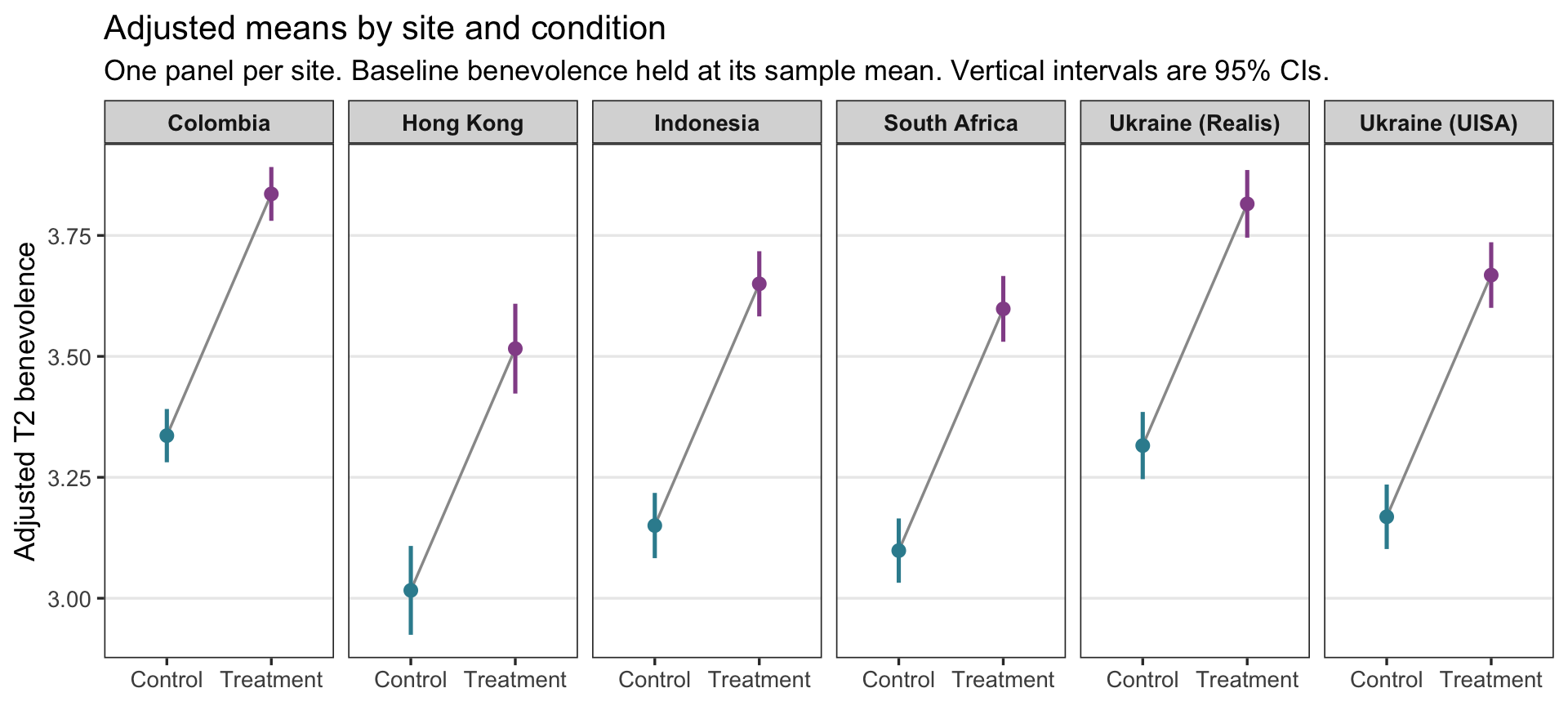
The sites sit at different heights, but every gray line rises by the same amount.

Step 4 — Why the gap is the same at every site

Here is the model’s equation, with the site term written in words:

\[\widehat{\text{T2}}_i \;=\; b_0 \;+\; b_1 \cdot \text{T1.c}_i \;+\; b_2 \cdot \text{treat}_i \;+\; (\text{the coefficient for participant } i\text{'s site})\]

Try it before you open the answer. In M10 you rebuilt each site’s mean as \(b_0 + b_{\text{site}}\). Write the Control and Treatment predictions for a Hong Kong participant at the average baseline (T1.c = 0), then subtract them. What’s left?

• Control (treat = 0): \(b_0 + b_{\text{HK}}\) = 3.336 + (-0.320) = 3.016
• Treatment (treat = 1): \(b_0 + b_{\text{HK}} + b_2\) = 3.016 + 0.500 = 3.516

Subtract, and everything except \(b_2\) cancels. The Hong Kong term is in both predictions, so it raises or lowers both by the same amount; the baseline term \(b_1 \cdot \text{T1.c}\) is in both too. Only \(b_2 \cdot \text{treat}\) changes when treat goes from 0 to 1. The same cancellation happens at every site and every baseline value: site moves both predictions up or down together, and treatment adds the same \(b_2\) on top.

That is what this additive model assumes: the model-implied Treatment − Control difference in predicted average T2 is the same at every site and every baseline value. It does not assume that every individual would experience exactly the same treatment effect. And it’s an assumption, not a finding. The model imposes a common gap, so the table and the figure display the assumption rather than test it. (A model that lets the treatment effect differ by site is a moderation model, which PSY 653 takes up.)

The answer to report

So in this model the estimand needs no extra calculation. The adjusted treatment effect is the treatment coefficient: 0.500 benevolence points, 95% CI [0.449, 0.550], the same model-implied contrast at any site and any baseline value. It is an assignment-based, complete-case contrast²: everyone is analyzed in the arm they were assigned to, but only participants with a T2 score are included. This is the central substantive finding of the analysis.

TipGoing further — averaging over the sample’s own sites

Step 2 pinned one site. A second way to get adjusted means from this model is to pick no site at all and let every participant keep their own. The question becomes: “if every participant in the analysis sample had been assigned to Control, what average T2 would the model predict? And if every one of them had been assigned to Treatment?” Those are two hypothetical versions of the same 3,965 people, identical except for the arm they’re assigned to — exactly the comparison the trial was designed to make.

Building them takes three verbs you already have. mutate() can overwrite an existing column, so make two copies of analysis with treat set to one value in each; predict() returns one prediction per row; mean() averages them:

everyone_control <- analysis |>
  mutate(treat = "Control")

everyone_treatment <- analysis |>
  mutate(treat = "Treatment")

pred_control <- predict(m2, newdata = everyone_control)
pred_treatment <- predict(m2, newdata = everyone_treatment)

mean(pred_control)

[1] 3.20894

mean(pred_treatment)

[1] 3.708654

# The average of each participant's Treatment − Control difference:
mean(pred_treatment - pred_control)

[1] 0.499714

The averaged adjusted means are 3.209 under Control and 3.709 under Treatment. They differ from Colombia’s (3.336 and 3.836) because they describe the sample’s mix of sites, each weighted by its share of the complete-case sample, rather than one site. But the averaged difference is 0.500, the same \(b_2\) again: averaging a column of identical differences returns that difference. (For the two averaged means, mean() gives the estimates but not their standard errors; the spread of participants’ predictions is not the standard error of an estimated average.)

In an additive model, the profile route and the averaging route always agree on the contrast. Once treatment interacts with another predictor, a contrast for one profile and the sample-average contrast can differ, and then this averaging route becomes the natural way to describe the trial’s sample as a whole.

APA-style reporting · the estimand-first version

APA-style reporting · Multiple Linear Regression (with site), estimand framing

A multiple linear regression was used to estimate the average effect of assignment to treatment on 2-week follow-up benevolence (an assignment-based, complete-case contrast among participants with observed T2), adjusting for centered baseline benevolence and study site. Participants assigned to the workbook scored an estimated 0.500 points higher on T2 benevolence than participants assigned to Control, holding baseline benevolence and site constant, SE = 0.026, 95% CI [0.449, 0.550], t(3957) = 19.31, p < .001. The causal interpretation of this contrast additionally depends on assumptions about missing follow-up outcomes. The overall model accounted for a substantial share of outcome variance, F(7, 3957) = 376.3, p < .001, R² = .400, adjusted R² = .399. The site block, included because site was the randomization stratum, accounted for additional variance beyond the baseline-and-treatment model, ΔR² = .011, F(5, 3957) = 14.1, p < .001. Site-level coefficients are not interpreted substantively (cf. Westreich & Greenland, 2013).

Note the structure: the adjusted treatment effect (the focal estimand) with its CI, t, and p comes first → then the model as a whole (omnibus F with df, R², adjusted R²) → then the site block (ΔR² and its nested-model F-test) → and an explicit note that control-variable coefficients are not interpreted (the slope on baseline benevolence stays in the regression table, not the paragraph).

---

Part 6 — Two jobs, and what licenses a causal claim

Two jobs for multiple regression

Everything in this Module has used multiple regression for one job: estimating a quantity the research question names, the treatment contrast, as precisely and honestly as the design allows. The M11 lab uses the same lm(), the same output, and the same inference recipe for a different job: building a model that predicts an outcome, in its case U.S. presidential vote shares, including for elections the model hasn’t seen. Gelman, Hill, and Vehtari list both among the most important uses of regression: prediction, “modeling existing observations or forecasting new data,” and causal inference, “perhaps the most important use of regression,” estimating treatment effects. Their very first example, in Chapter 1, is the election-forecasting model the lab builds on: vote share predicted from economic growth.

Same model, two jobs

	Estimating a focal quantity (this Module · REACH)	Building a prediction model (the M11 lab · Bread + Peace)
The question	How much higher is T2 benevolence for participants assigned to the workbook, compared with people at the same site who start at the same baseline benevolence?	How well do economic growth and military fatalities predict the incumbent party’s vote share?
What you report	One estimand — the treatment contrast — with its CI	Predictions for new cases with prediction intervals, plus how well the model fits (R², \(\sigma\))
Why each predictor is there	The design: baseline benevolence sharpens precision; site is the randomization stratum	The substantive theory, and how much each predictor improves the predictions
The other coefficients	Supporting detail, not read causally (the Table 2 fallacy)	Each one describes an adjusted association; none can be read as a causal effect, because nothing was randomized
What to watch for	Adjusting for a post-treatment variable; causal language the design doesn’t support	Trusting a forecast beyond the range of the data; with only 17 elections, precision is limited and one election can change an estimate a lot

The two columns overlap: a prediction model’s coefficients are still adjusted comparisons, and an estimand model still makes predictions. What changes is which output you lead with, and which mistakes you guard against.

Prediction vs causation

In the REACH analysis, the treatment coefficient stays about half a benevolence point in both multiple-regression models. Because REACH was a randomized controlled trial, that coefficient has a causal basis that an observational comparison lacks. Random assignment ensures that, in expectation, the randomized treatment and control groups are equivalent on every variable — measured and unmeasured — at baseline. One caveat matters here: our analysis uses only participants with an observed T2 score, and follow-up completion happens after randomization. Completers were still assigned at random, but the complete-case subsets need not retain the comparability (exchangeability) that randomization created in the full randomized sample, so the causal reading additionally depends on assumptions about why people did or didn’t complete follow-up. (The published REACH analysis used multiple imputation in an intention-to-treat framework; those methods address missing outcomes under their own assumptions, rather than automatically eliminating all possible missing-data bias.)

If the same regression were run on observational data — for example, comparing people who had chosen to use a forgiveness workbook to people who hadn’t — the same coefficient could not be read as a causal effect. People who choose forgiveness workbooks differ from people who don’t on dozens of characteristics: openness, current relationship distress, religious affiliation, income, time available. The treatment coefficient in an observational analysis bundles together the workbook’s actual effect and all of those pre-existing differences between the two groups. In an observational study, adjusting for appropriate measured pre-treatment confounders can reduce that bundling — but ordinary regression adjustment cannot directly control confounders you did not measure.

This distinction is sometimes summarized as: regression as prediction vs regression as causal inference. Both use the same lm() syntax and produce the same kind of output. What differs is the research design that generated the data, and therefore what the coefficients are entitled to mean.

What licenses a causal interpretation?

Design	What the treatment coefficient means	Causal interpretation?
RCT (REACH)	Average causal effect of assignment to the intervention on benevolence	Yes, by random assignment (our complete-case version adds an assumption about missing follow-ups)
Observational (e.g., self-selected workbook users vs non-users)	Predicted post-test difference, given the way users and non-users differ in the data	No, unless you can rule out unmeasured confounders
Natural or quasi-experiment with as-if-random assignment	A causal estimand that depends on the design	May be warranted, if the identifying assumptions hold

In this Module’s REACH analysis, a careful sentence is: “Among participants with follow-up data, those randomly assigned to the workbook scored an estimated 0.50 points higher on T2 benevolence, adjusting for baseline benevolence and site.” Randomization gives that difference a causal basis; the complete-case restriction is the reason to state it this carefully. If you do regression on observational data later in your career, be careful with causal language — the same lm() output supports a predictive statement but not a causal one.

For a total treatment effect, prefer appropriate pre-treatment controls over variables affected by treatment

The baseline-adjusted and site-adjusted models adjust only for a variable measured before randomization (baseline benevolence) and one fixed by the design (site). That’s deliberate. Gelman, Hill, and Vehtari warn that “it is generally not a good idea to adjust for variables measured after the treatment.” Suppose we added a measure taken at the 2-week follow-up, such as empathy toward the offender. The workbook may change empathy, and empathy may change benevolence. Adjusting for it would compare Treatment and Control participants with the same post-workbook empathy — taking away part of the workbook’s effect, and comparing groups that are no longer randomized with respect to that variable. Questions about how an intervention works (mediation) need their own designs and assumptions, which more advanced courses take up.

Model building — a brief field guide

Two models ago we had t2 ~ treat. Now we have t2 ~ baseline + treat + site. We could keep adding predictors — age, religion, sex, education, marital status, ethnicity — and the model would keep gaining R². Should we?

A short field guide for deciding, following the principles in Regression and Other Stories:

1. Include predictors for substantive reasons. Each predictor should be justified by the research question or the design, not be in the model “because it’s available.” Baseline is in because it’s a strong pre-treatment predictor of the outcome; site is in because it is the randomization stratum; marital status would need its own justification.
2. Don’t choose predictors by statistical significance. A predictor that matters for the question can stay in the model even if its estimate has a large standard error; dropping or adding predictors because of their p-values makes the results hard to interpret.
3. For estimating a total treatment effect, generally adjust for appropriate pre-treatment variables rather than variables affected by treatment (the section above).
4. Sample size should follow the estimand. There is no universal “observations per predictor” rule that guarantees a good regression. Planning depends on the precision or power you need for the focal estimand, the number of predictors and how strongly they correlate, and the model you intend to fit. For important studies, use a design-specific power or simulation analysis, as in M07–M09, rather than a fixed ratio.
5. Highly correlated predictors make their individual coefficients unstable, and that instability shows up as large standard errors. M12 shows how to check.
6. Record, and when you can pre-register, your modeling choices. If the regression is the primary analysis for a study, specify the predictors before you see the outcomes, so analytic flexibility doesn’t turn into an unintentional search for a result. Tools for choosing among candidate models when prediction is the goal (AIC, BIC, cross-validation) come in more advanced courses.

The REACH analyses in this Module use a small, theoretically motivated set of predictors: baseline benevolence (a strong pre-treatment predictor of the outcome), treatment (because it’s the focal predictor), and site (because it is the randomization stratum). That’s a coherent model-building rationale, articulable in two sentences. Reach for the simplest model that answers the question you’re actually asking, then report whichever quantity answers it directly: a coefficient or a model-based comparison.

---

Looking ahead

You’ve now built two MLRs and reported each by starting from the estimand. The progression:

Model	Specification	What the model is for	The focal estimand
Treat-only (SLR, M10)	t2 ~ treat	Simplest two-group comparison	Raw mean difference
M11 baseline-adjusted (MLR)	t2 ~ t1 + treat	Adjust for baseline benevolence — precision gain	Adjusted treatment effect at the same baseline benevolence
M11 site-adjusted (MLR)	t2 ~ t1 + treat + site	Align with the within-site randomization; absorb between-site mean differences	Adjusted treatment effect, the same at every site and baseline value (an additive model)

Each step refines how we estimate and express the randomized treatment contrast, without leaving lm(). The focal-estimand column is the substantive thing each model is built to estimate — not the per-coefficient table dressed up as a series of findings.

The model with site is the specification we carry into M12. A fitted model is still a claim about how the data behave, so M12 takes that exact model and audits it: the residual–fitted plot (linearity and equal variance, including the bounded-outcome wedge that REACH makes especially vivid), Q–Q plots, influence diagnostics such as Cook’s distance and leverage, the variance inflation factor for multicollinearity, and a remediation toolkit for when an assumption doesn’t hold. Fit → query → check.

Going forward, regression extends in directions you’re likely to meet next:

• Moderation (effect modification). When the treatment effect depends on a third variable (baseline benevolence, age, site), a single treatment coefficient stops being the right summary. PSY 653 introduces interaction terms (treat * baseline) and the tools for probing how an effect changes.
• Good and bad controls. Not every “control variable” makes a regression cleaner — some controls introduce bias (collider control), and some control away the very effect you’re trying to estimate (over-control). The causal-diagram (DAG) framework is the tool that distinguishes them, and it formalizes the Table 2 fallacy.
• Non-linear effects and model selection. “Linear” regression means linear in its parameters, so curves fit inside the same framework: a quadratic term such as I(t1_benevolence^2), splines, generalized additive models, and transformations. Regularization, AIC/BIC, and cross-validation help choose among models. More advanced courses develop these tools.

The same M11 sequence — define a target, fit a suitable model, and get an interpretable estimate from it — carries through every one of these extensions.

Summary

Core ideas: Multiple Linear Regression

1. In the additive models we fit in M11, each MLR coefficient is an adjusted comparison. \(b_j\) is the predicted difference in \(y\) between two people one unit apart on \(x_j\) who have the same values on the other predictors — what “holding constant” means in practice. It compares people; it doesn’t describe one person changing. A causal interpretation needs design or identification assumptions: in REACH, random assignment supports an average causal interpretation of the Treatment–Control contrast, not any one person’s treatment effect.
2. Residualized gain is the conceptual on-ramp. Fit t2 ~ t1, examine the residuals by treatment, and the difference of mean residuals closely previews the MLR treatment coefficient (the exact version residualizes both sides). The one-step lm() does the same arithmetic with the right degrees of freedom. Subtracting baseline benevolence instead (a gain score) assumes a slope of 1; the regression estimates it.
3. Centering moves the intercept’s meaning, not the model. Subtracting a predictor’s mean shifts the intercept from “predicted \(y\) at \(x = 0\)” to “predicted \(y\) at the average \(x\),” with no change to slopes, R², or \(\sigma\).
4. Adding a strong pre-treatment covariate can raise precision without changing what a randomized comparison estimates. Here baseline benevolence does so substantially because it is strongly prognostic and nearly unrelated to treatment. Because random assignment balances covariates across arms in expectation, adjustment shouldn’t systematically shift the treatment-effect estimate; in a given sample it barely moves, while the SE shrinks because the residual variance shrinks.
5. R² and adjusted R². R² never falls when a predictor is added; adjusted R² penalizes extra predictors. A small R² is not a flaw, and R² depends on how spread out the predictors are in the sample.
6. Start with the estimand, not the coefficient table. Name the quantity the research question asks for, then get it from the model. In these additive models the treatment contrast equals the treatment coefficient; predict() with interval = "confidence" gives adjusted means for profiles you name (with a categorical predictor, the profile has to name a category). In richer models the estimand may require combining several predictions, so the habit matters more as models grow.
7. Categorical predictors with \(L\) levels generate \(L - 1\) dummies. The intercept becomes the reference-group adjusted mean; each dummy’s coefficient is its category’s adjusted-mean difference from the reference.
8. Site is a randomization stratum and a source of systematic mean differences. Site dummies in REACH account for between-site mean differences and align the model with the within-site randomization; they do not by themselves guarantee independent residuals within site. This site-as-predictor form is the fixed-effects approach; with only six sites it is a simple, transparent adjustment, and multilevel (mixed-effects) models, which partially pool sites toward a common distribution, are the fuller framework, covered in PSY 653.
9. A coefficient can change when a predictor is added, because the comparison it makes changes. Part of a raw gap can be carried over from the added predictor. Randomization made that tiny for treatment; the site gaps shrink once baseline benevolence enters, because the sites started at different baseline levels.
10. ΔR² and the nested-model F-test. ΔR² is how much a predictor or block adds to R², always relative to a stated smaller model (for one predictor, psychology’s squared semi-partial correlation \(sr^2\)). The nested-model F-test asks whether the addition is larger than sampling noise would tend to produce.
11. The Table 2 fallacy. Control-variable coefficients are conditional association parameters that help isolate the focal contrast; they are not automatically causal effects of the controls themselves. Report estimands, not coefficient tables dressed up as findings. For the total treatment effect, do not naively adjust for variables affected by treatment: doing so can block part of the effect or introduce bias.
12. Random assignment is what supports a causal interpretation. The REACH treat coefficient has a causal basis because the trial randomized; restricting to participants with follow-up data adds an assumption about missingness. The same lm() output from observational data would describe a predicted difference, not a causal effect.

Credits

• The reach_analysis data are a course-prepared subset of Ho, Worthington, Cowden, et al. (2024), International REACH forgiveness intervention: a multisite randomised controlled trial (BMJ Public Health).
• These Module materials draw on Gelman, Hill, & Vehtari’s excellent book Regression and Other Stories (2020, Cambridge University Press), which the authors make free to view for personal use from the book’s web page. It’s a strong next step for going deeper into Part 3’s regression material.
• The Module’s approach was also shaped by Richard McElreath’s Statistical Rethinking (2nd ed., 2020, CRC Press) and, more broadly, by his approach to teaching statistical modeling.
• The estimand-centered framing follows Rohrer & Arel-Bundock (2026).

Footnotes

1. Unbiased for the causal effect of treatment by design, setting aside follow-up missingness. Adjusting for site isn’t required for that unbiasedness — treatment was randomized within site — but it sharpens precision and aligns the estimand with the blocking structure, as Part 4 develops.

2. Intention-to-treat (ITT) analyzes each participant in the arm they were randomly assigned to, whether or not they completed the workbook. It estimates the average effect of being assigned to treatment, the quantity randomization protects from confounding, and it is the headline estimand most trials report (see the CONSORT reporting guideline). Restricting to participants with an observed outcome is a separate, complete-case issue, which is why our contrast is assignment-based but not strict ITT.