Confidence Intervals
Pre-Study · Module 7 · Fri Sep 25
Welcome to the M07 pre-study. You’ve already read the M07 Module — the one-sample problem, bootstrap percentile CIs, parametric t CIs, the long-run interpretation of 95%, and the CI-vs-PI distinction. That was the textbook treatment. This pre-study is where four things click into place with hands-on practice.
You’ll feel the 95% long-run interpretation in an in-browser simulator. You’ll watch the key concepts narrated with visuals. You’ll practice the core infer R moves — rep_slice_sample() + quantile() for the bootstrap and t_test() for the parametric shortcut. And you’ll close by building both a confidence interval and a prediction interval.
How this page is organized
Four short videos drive home the Module’s hardest conceptual moves. After Video 1 you’ll walk through an interactive simulator. After Videos 2 and 3, you’ll build two 95% CIs in R — one via the bootstrap and one via the parametric t formula. After Video 4 you’ll build a CI and a PI side by side from one sample, so the CI-vs-PI distinction stops being an abstraction.
Every code activity uses a three-tab panel:
- ✍️ Your Code — the starter with blanks for you to fill in
- 💡 Hint — a nudge in the right direction
- 👀 Spoiler — the full working code if you get stuck
Work through the ✍️ tab first. Only open 💡 or 👀 after you’ve tried it yourself — struggling a little is how this stuff sticks. Plan on about 90 minutes for the whole page.
The college_mobility dataset
The pre-study uses the same dataset as the M07 Module: 2,199 U.S. colleges with median earnings at age 34 for the cohorts that attended them (Chetty et al., 2017). The dataset is already loaded into your sandbox under the name college_mobility, and tidyverse is attached — so every chunk on this page can reference college_mobility without any setup on your part.
college_mobility · 2,199 observations · 2 variables · Chetty et al. (2017)
- name character — Institution name
- k_median numeric — Median individual earnings, in 2014 US dollars, among the college’s former students
The teaching trick: because this is the full population of U.S. colleges with adequate data, we know the true population mean is $36,929. Every CI you build in this pre-study can be checked against that truth — a luxury real research never has.
Full codebook for college_mobility — values, levels, missingness, and how the file was prepared.
Want to confirm the data is loaded? Run the chunk below — glimpse() prints one row per variable with the variable type and first few values.
Video 1 — What a 95% Confidence Interval Actually Means
What to listen for:
- A CI is a range built from one sample to describe a population parameter
- The 95% describes the long-run performance of the procedure, not this specific interval
- The classic misinterpretation: “there’s a 95% probability the true mean is in this interval” — named explicitly and rejected
- The trade-off: 90% vs. 95% vs. 99% CIs — higher confidence buys coverage at the cost of width
Interactive: see 95% in action
The long-run interpretation is slippery on a first reading. A simulator built by Dr. Kristoffer Magnusson makes it visible: it draws sample after sample, builds a confidence interval from each, and keeps a running tally of how often those intervals capture the true mean.
Open it in a new tab now and keep it beside this page — you’ll get your bearings with the screen map below, then run four short prompts against it.
Open the simulator in a new tab
rpsychologist.com/d3/ci
What you’re looking at
This is a generic teaching simulator — its population is centered at μ = 0, not our college-earnings data. That’s the point: what “95%” means is universal, and a clean μ = 0 makes it easy to see. Use the red vertical dashed line at μ = 0 as your anchor — intervals that cross it capture the truth; intervals that miss it (drawn in red) do not.
Screen map — what each part means:
- Top slider (“Slide me”) = confidence level (50%, 95%, 99%).
- Bottom controls = sample size (\(n\)) and run/pause speed.
- Main CI panel = one interval per sample; red intervals are misses (they do not include μ — the true population mean).
- Left dials = running totals and coverage: μ included, μ missed, and CI coverage (%), computed as \(\mu\ \text{included} /(\mu\ \text{included} + \mu\ \text{missed}) \times 100\).
- Middle-left line plot (Proportion of CIs that include population mean) = the running coverage rate; with enough samples it settles near your chosen confidence level.
- Bottom-left distribution (CIs sampling distribution, x-axis = CI Width) = how much interval widths vary from sample to sample (width = upper bound − lower bound, not where the sample mean sits).
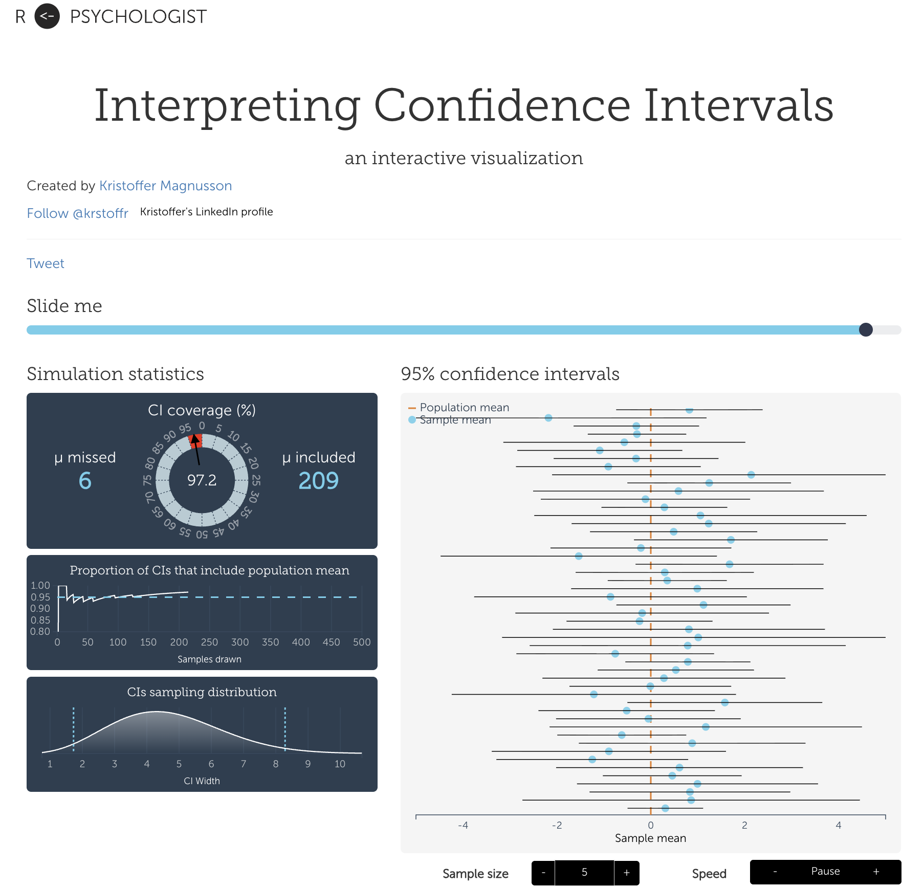
Before the prompts, just let it run for a minute and watch: red vs. non-red intervals appearing in the main panel, and the coverage curve drifting toward your chosen confidence level. Once that clicks, you’re ready.
How to run each prompt
The left-side dials and line plot finalize their readings only when you click Pause. So every prompt uses the same rhythm:
- Set the confidence level and sample size the prompt asks for.
- Unpause / Play, and let it run ~30 seconds so plenty of samples accumulate.
- Pause, then read the numbers off the left-side dials.
That set → run → pause → read loop applies to all four prompts. Work them in order — we won’t repeat the rhythm in each one.
Prompt 1 (Baseline). Set sample size = 150 and confidence = 95%. Estimate the miss rate — what percent of intervals are red (miss \(\mu\))? You can compute this as \(\mu\ \text{missed} \;/\; (\mu\ \text{missed} + \mu\ \text{included}) \times 100\), or more simply as \(100 - \text{CI coverage (\%)}\).
Prompt 2 (Change confidence only). Keep n = 150. Lower the confidence level to 50%. Compared to Prompt 1, what happens to the CI width and the miss rate?
Prompt 3 (Change sample size only). Return confidence to 95%. First set n = 15 and observe. Then increase to n = 100 and observe. Comparing the two settings, what changes about the CI width and what stays about the same about the miss rate?
Prompt 4 (Single-interval interpretation). Pick one red interval from the main CI panel. True or False: If the red dashed \(\mu\) line were hidden, you could tell from that interval alone that it had missed.
What the simulator just taught you
The two knobs are independent. Confidence level and sample size control different things, and the simulator let you move each on its own:
- Confidence level sets the hit rate (calibration). A 50% CI misses ~half the time; a 95% CI misses ~5% of the time — the number in the label is the long-run coverage rate, and 100 minus it is the long-run miss rate.
- Sample size sets the width (precision). Bigger \(n\) narrows the intervals without changing how often they miss. The two knobs trade off on different axes.
Running coverage settles. The middle-left Proportion of CIs that include population mean line plot stabilizing near the nominal level is the Law of Large Numbers from M06 in action — this time applied to the success rate of the procedure itself, not to a sample mean. Short runs wobble; long runs converge.
Misses are unbiased random bad luck, not systematic error. The red intervals in the main panel scatter both above and below \(\mu\) in roughly equal numbers. A missed CI isn’t evidence of a flawed sample or a broken method — it’s just a 5%-probability event that happened this time.
The a-ha moment
Every “95% CI” you will ever read in a published paper is a single draw from the process you just watched. It might be one of the 95 that caught the truth. It might be one of the 5 that didn’t. Nothing about the interval itself — its width, its bounds, its center — tells you which.
So when someone says “we are 95% confident the true effect lies between 0.12 and 0.38,” notice the sleight of hand: they are borrowing the reliability of the procedure (which catches the truth 95% of the time over many studies) and silently attaching it to this one interval (which either caught it or didn’t — we can’t know).
Your confidence lives in the method, not in the numbers on the page. Once you see it this way, you can’t unsee it.
Quick Check
Answer each question — you’ll see green (correct) or pink (incorrect) feedback as you type.
1. The simulator you ran above draws a fresh sample and builds a new 95% CI from it, over and over. Suppose you let it run at 95% until the μ included and μ missed dials together reached 500 intervals. Roughly how many of those 500 should include μ?
2. A colleague writes in a draft: “The 95% CI for the effect was [0.12, 0.38], meaning there’s a 95% probability the true effect lies between 0.12 and 0.38.” Which statement is true?
3. True or false: Widening a CI from 95% to 99% makes the interval wider but also makes it more likely, in the long run, to capture the parameter.
4. You look at a published 95% CI of [0.12, 0.38]. Can you tell from this interval alone whether it actually captured the true effect?
Defining the sample
For the rest of this video series, we’ll work with our researcher’s sample of 50 colleges and walk through how to build a confidence interval — first using a bootstrapping approach, then using a parametric approach. One thing to flag before we dive in. In the Module reading, we worked with a sample of 250 colleges. Here in the videos, we’re going to scale that down to a sample of 50. And that gives us a chance to see something important — a smaller sample produces a wider confidence interval. The intervals we build here will come out looser than the Module’s — nearly twice as wide, mostly the price of the smaller \(n\), though the two draws’ particular spreads contribute a little too — and watching that difference show up is part of the lesson.
Video 2 — Bootstrap Resampling
What to listen for:
- Bradley Efron’s insight: treat your sample as a mini-population and resample from it
- Why sampling with replacement is non-negotiable — without it, every resample is identical
- Running the resample 1,000 times produces the bootstrap distribution
- The middle 95% of that distribution is the 95% CI — read the bounds off with quantile(), not qnorm()
Warm-up: what does “with replacement” actually look like?
Before we scale up, let’s see one resample on a tiny example. Run this chunk a few times — notice which values repeat and which drop out.
Each resample has the same 10 values available, but some repeat and some don’t appear at all. That variation is what the bootstrap is after — it mimics what different real samples might have looked like if we could have drawn them from the population. Now let’s scale up.
Activity 2.1 — One resample, one mean
We’ll draw one sample of 50 colleges from college_mobility, then draw one bootstrap resample from it. Your task: fill two blanks — one to compute the mean of the original sample, one to make the resample use replacement.
The first blank takes a base-R function that computes an arithmetic average. The second blank is the logical value that turns on sampling with replacement.
Your two numbers should be close but not identical. The original sample mean is your point estimate; the resample mean is one plausible alternative. Do this 999 more times and you have the bootstrap distribution. (Not really — we’ll automate it with rep_slice_sample() in the next activity.)
Activity 2.2 — 1,000 bootstrap resamples with rep_slice_sample()
Now automate the “draw a resample, compute its mean” loop 1,000 times. The rep_slice_sample() function from the infer package is slice_sample() repeated many times: with reps = 1000 it draws 1,000 independent resamples and stacks them into a single tibble, adding a replicate column that labels each row with which resample it came from. Follow that with group_by(replicate) |> summarize() and you get one mean per resample — the bootstrap distribution.
Your task: fill two blanks — how many resamples to run, and which column to group by.
The bootstrap is robust at 1,000 resamples — enough that running again produces nearly the same CI, not so many that you wait. Type 1000 for the first blank. For the second, rep_slice_sample() adds a column called replicate — that’s the one to group by.
You’ve built the bootstrap distribution. Each row of bootstrap_samples is one bootstrap resample’s mean.
What you see is not all you have. head() prints only the first six means, so the output stays readable — but the tibble holds all 1,000, which is exactly what the nrow() line underneath is confirming. Every step from here — the standard error in Activity 2.3, the percentile interval in Activity 2.4 — is computed from all 1,000 means, not from the handful on screen.
What rep_slice_sample() just did
rep_slice_sample() is slice_sample() repeated reps times, with one addition: it stamps each resampled row with a replicate column so you know which resample it came from.
my_sample |>
  rep_slice_sample(n = 50, replace = TRUE, reps = 1000)
#> A tibble with 50 × 1000 = 50,000 rows, plus a `replicate` column 1..1000
After that call, every row is one college pulled into one of the 1,000 resamples. To turn those into 1,000 sample means, group by replicate and summarize:
|> group_by(replicate) |> summarize(mean_income = mean(k_median))
#> A tibble with 1,000 rows — one mean per resample
That tibble is the bootstrap distribution. The column mean_income holds all 1,000 bootstrap means, ready for sd() and quantile() in the next two activities.
Activity 2.3 — Standard error: the SD of the bootstrap distribution
You’ve got 1,000 bootstrap means — one number per resample. Their spread tells you how much the sample mean would wobble if you could really repeat the experiment many times. The standard deviation of the bootstrap distribution has a name: the standard error (SE) of the mean.
Compute it now. And compare it to the SD of the data itself — they measure two different spreads.
Your task: fill the single blank with the function that computes a standard deviation. The contrasting SD of the data below is written for you.
Both blanks call the same R function — sd() computes a standard deviation. What changes is what’s inside: the SE is the SD of the bootstrap means; the SD-of-data is the SD of the individual k_median values.
You should see the SE come out around $1,500 and the SD of the data around $11,000 — roughly seven times larger. Both are “spread” numbers, but they describe different spreads. The SE is the spread of the sample mean across hypothetical repeats; the SD-of-data is the spread of individual colleges within one sample. Most of the noise in your data is between-college variation; what’s left after averaging across 50 of them is the SE.
SE vs SD — the most-confused pair in introductory stats
When a paper reports a mean ± something, the “something” is almost always the standard error, not the standard deviation:
- SD-of-data — how much individual cases differ from the sample mean. Tells you the spread of the data.
- Standard error (SE) — how much the sample mean itself varies across hypothetical repeats. Tells you the precision of an estimate.
The SE is smaller than the SD-of-data by about a factor of \(\sqrt{n}\) — exactly \(\sqrt{n}\) for the parametric formula you’ll meet in Video 3, and close to it for the bootstrap estimate you just computed, which carries a little simulation noise of its own. Larger samples shrink the SE (your estimate is more precise) without affecting the SD-of-data (the variability of cases is what it is). When you see “M = 37.1, SE = 1.5” in a results table, that 1.5 is the same kind of bootstrap-style spread you just computed.
You’ll meet the SE again in Video 3 as \(s/\sqrt{n}\) — the parametric shortcut to the same number, no resampling required.
Activity 2.4 — Read the 95% CI off the bootstrap distribution
The middle 95% of the bootstrap distribution is your 95% CI. quantile() gives you the cutoff at any percentile. For 95% you want the 2.5th and 97.5th percentiles — 2.5% in each tail.
Your task: fill the two probs blanks — the percentiles marking the lower and upper bounds of a 95% interval.
A 95% CI excludes 5% — 2.5% in each tail. So the lower bound is at the 2.5th percentile (0.025) and the upper bound is at the 97.5th percentile (0.975).
That’s your 95% bootstrap percentile CI. The true population mean of college_mobility is $36,929 — check whether your interval contains it. If it does, your method worked on this one run; if not, you’re one of the ~5% of intervals that misses. That’s 95% in practice.
Now see it. Your interval is nothing more than two cutoffs on the distribution you built in Activity 2.2. Run the chunk below to draw them — it rebuilds the figure from Video 2, using your numbers.
Three things to read off it. The lavender lines are your lower and upper — 950 of the 1,000 resample means sit between them, which is what “95%” means here. The rose line is your sample mean, and the bootstrap distribution is centered on it, not on the truth. The gold line is the true \(\mu\) — visible only because college_mobility is the whole population, and the one thing real research never gets to draw.
Video 3 — The t-Distribution and its Critical Values
What to listen for:
- We use t, not z, because \(\sigma\) is estimated from the sample with s — which is itself noisy
- Degrees of freedom (\(df = n - 1\)) control the t-distribution’s shape — heavier tails for small n, tight normal-like for large n
- qt() is qnorm()’s sibling — same what-cuts-off-this-percentile? logic, different reference distribution
- The parametric formula: \(\bar{x} \pm t^* \cdot s/\sqrt{n}\)
First, the words: critical value, and the star
A critical value is a cutoff on a reference distribution — the point that fences off a chosen amount of area under the curve. For a 95% CI you want the middle 95%, so the two cutoffs leaving 2.5% in each tail are the critical values. That is exactly what qnorm() and qt() hand you.
Its symbol carries a star — \(z^*\) read off the normal curve, \(t^*\) off the t curve — and the star is what marks it as a critical value. Keep that separate from plain \(t\):
- \(t\) is where your sample landed. It comes from your data, and a different sample gives a different \(t\).
- \(t^*\) is where you drew the fence. It comes from your choice of confidence level (plus \(df\)), and your observed values never touch it.
You never actually compute \(t\) in this Module — \(\mu\) sits in its numerator, and \(\mu\) is the unknown. The only number you calculate is \(t^*\). The Module works all of this through in full; this is the short version, so the activities below make sense.
Activity 3.1 — Compare t and z critical values
Run the chunk and watch the pattern. Four numbers: the standard-normal (z) critical value for 95%, and the t critical value at three sample sizes.
Notice the pattern. The z cutoff is fixed at 1.96. The t cutoffs start larger (df = 10 → ~2.23) and shrink toward 1.96 as df grows. That’s the t’s heavier tails accounting for the fact that we estimated \(\sigma\) with s — and the tails collapse onto the normal as the sample grows and s becomes a more reliable stand-in for \(\sigma\).
Activity 3.2 — Build a parametric 95% CI by hand
This is the by-hand version of the formula your Monday lecture uses — the exact pipeline the M07 Module walked through. A single summarize() call computes every piece of the CI in one expression.
Your task: fill the four blanks so the pipe computes, in order — the sample mean and standard deviation of k_median (first two blanks), the degrees of freedom \(n - 1\) (third blank), and the t critical value at the 0.975 percentile (that’s 2.5% in each tail for a two-sided 95% CI — not 0.95; fourth blank). The se, lower, and upper lines are already wired up from those pieces.
- The first two blanks are base-R functions for mean and standard deviation.
- n() inside summarize() returns the number of rows in the group — that’s your \(n\).
- For a 95% CI you want the cutoff at the 0.975 percentile (2.5% in each tail).
- Degrees of freedom: \(df = n - 1\).
Your parametric 95% CI should be very close to — but not identical to — the bootstrap CI from Activity 2.4. Two different construction methods, same sample, similar answers. That’s the reassurance the Module made explicit: when the CLT applies, the bootstrap and the parametric approach should agree.
Activity 3.3 — The t_test() shortcut
In practice, nobody hand-computes \(\bar{x}\), \(s\), \(\text{SE}\), and \(t^*\) every time. The infer package wraps the whole pipeline in a single t_test() call.
Your task: fill two blanks — response is k_median — the earnings column you’ve been building CIs for — and conf_level is the confidence level written as a proportion, 0.95 (not 95).
- The response variable is the numeric column whose mean you want a CI for — the same column you used in Activities 3.1 and 3.2.
- For a 95% CI, conf_level is
0.95(a proportion, not a percent).
Compare the lower_ci and upper_ci you just got to the lower and upper from Activity 3.2’s hand-computed parametric_ci. They should be identical — t_test() is running the exact same formula under the hood.
The columns you selected:
- t_df — degrees of freedom (\(n - 1\))
- estimate — the sample mean \(\bar{x}\)
- lower_ci / upper_ci — the 95% CI bounds
Learn the by-hand version first so you understand what t_test() is doing — but after that, reach for the shortcut. This is the calculation you’ll most often use in practice.
Quick Check
Answer each question — you’ll see green (correct) or pink (incorrect) feedback as you type.
1. With a sample of \(n = 50\), what are the degrees of freedom for the t-distribution used in a 95% CI for the mean?
2. Why do we use the t-distribution instead of the normal when constructing a CI for a mean?
3. For a large sample (say \(n = 500\)), the t critical value for a 95% CI is closest to —
Video 4 — When You Care About One New Case
What to listen for:
- The CI and PI answer different questions from the same sample — where is the population mean? vs. where might a single new case land?
- The PI uses \(s\) itself, not \(s/\sqrt{n}\) — so outcome variability does not shrink as \(n\) grows
- The PI is essentially the M06 empirical rule (\(\bar{x} \pm 2 \cdot s\)), sharpened with \(t^*\) and a small finite-sample correction
- For the same sample, the PI is roughly seven times wider than the CI — and one of them may be more decision-relevant for your reader
The activities below put both intervals side by side from one sample, so you can see — in dollars — how much wider the PI is and verify that it really does cover ~95% of individual colleges.
Why this matters for psychology students
Reading a CI correctly is one professional skill. Knowing when a CI is the wrong tool and you need a prediction interval (PI) instead is another — and it’s the one the Zhang et al. (2023) physicians really missed. Three things you should be able to do by the end of these activities:
- Build both intervals from the same sample. One summarize() call, side by side — the CI and the PI come out together.
- See that the PI is always wider. For the same confidence level and sample, the extra “+1” under the PI’s square root guarantees it. About how many times wider?
- Verify PI coverage empirically. Because we have the full population, we can count: what fraction of the 2,199 individual colleges actually fall inside the 95% PI? It should be near 95%, and the small deviation will tell you something honest about distributional assumptions.
By the end of these activities, you’ll have the R pipeline and the intuition to not make the Zhang-physician mistake yourself.
Activity 4.1 — Build a CI and a PI in one summarize()
The Module’s CI and PI formulas differ by just one piece:
\[ \text{95\% CI for the mean:}\quad \bar{x} \pm t^* \cdot \frac{s}{\sqrt{n}} \qquad\quad \text{95\% PI for a new observation:}\quad \bar{x} \pm t^* \cdot s\sqrt{1 + \tfrac{1}{n}} \]
The PI has an extra “\(+1\)” inside the square root — the variance of a single observation around the mean. That piece is what makes the PI wider, and — unlike the CI — it keeps the PI from shrinking as \(n\) grows.
Your task: fill two blanks. The first completes the CI’s standard-error denominator. The second is the “\(+1\)” that turns the CI formula into the PI formula.
- The CI denominator is \(\sqrt{n}\) — the standard error of the mean is \(s / \sqrt{n}\).
- Inside the PI’s square root, add
1to \(1/n\) — that’s the variance of a single observation around the mean.
One sample, two intervals — the same center, very different widths.
Activity 4.2 — Compare the widths
The formulas guarantee the PI is wider. How much wider?
The ratio column tells you how many times wider the PI is than the CI. For \(n = 50\) it should be roughly 7×. That’s not a rounding artifact — it’s the quantified cost of asking “where is the next individual college?” instead of “where is the average college?”
Does that 7× hold for any sample size?
No — and the reason is the CI/PI distinction. Divide the two half-widths and both \(t^*\) and \(s\) cancel out:
\[\frac{\text{PI half-width}}{\text{CI half-width}} = \frac{t^*\,s\,\sqrt{1 + 1/n}}{t^*\,s/\sqrt{n}} = \sqrt{n+1}\]
The ratio depends on nothing but \(n\). At \(n = 50\) that is \(\sqrt{51} \approx 7.1\) — so the 7× above is a fact about this sample size, not about prediction intervals in general. Run this and watch it climb:
Why it climbs. As \(n\) grows the CI collapses toward zero — more data pins the mean down ever more precisely. The PI does not. Its half-width settles at \(t^* \cdot s\), the irreducible spread of individual colleges, which no amount of extra data can shrink. One shrinks to nothing, the other levels off, so the gap between them widens without limit. That is exactly the “PI levels off” line you saw in Video 4.
The practical version is worth carrying forward: collecting more data barely narrows a prediction interval. If you need to say where the next college will land, a bigger sample is not the fix — only less variable colleges would be.
Activity 4.3 — Does the PI actually capture ~95% of individual colleges?
A 95% PI built from one sample should cover about 95% of the individual colleges in the population — if the normality assumption holds. We happen to have the full population in college_mobility, so we can check that coverage directly.
Your task: take the PI bounds you just built, count how many of the 2,199 colleges have earnings (k_median) that actually fall inside those bounds, and turn that count into a percentage of all colleges — then compare it to 95%. The code below already pulls the bounds (pi_lo, pi_hi) and counts the colleges inside (n_inside_pi) and in total (n_total); you just fill in pct_inside, the percent inside.
The percent inside the PI is n_inside_pi divided by n_total, multiplied by 100 to display as a percentage.
You should land on 94% — close to 95%, but not exactly 95%. The college_mobility distribution is right-skewed (remember the histogram from the Module), and the PI formula assumes approximate normality. A little under-coverage is the data telling you, honestly, that distributional assumptions matter more for PIs than they do for CIs.
Quick Check
1. For the same sample and confidence level, the PI is always wider than the CI.
2. As \(n \to \infty\), what happens to the CI width and the PI width?
(Hint: the CI uses \(s/\sqrt{n}\), which vanishes as \(n\) grows. The PI uses \(s\sqrt{1 + 1/n}\), which approaches \(s\) — a finite width.)
3. A paper reports “a 95% CI of [0.32, 0.64] for the treatment effect.” From this CI alone, you can conclude that about 95% of individual patients will experience an effect between 0.32 and 0.64.
This is the Zhang-physician misreading. The CI tells you about the precision of the group-mean estimate, not about the range of individual outcomes. For the individual question, you need a PI — which would be considerably wider.
Four things to carry into lecture
- Every CI is built from one sample to describe a population parameter. The 95% describes the method, not this interval. The RPsychologist simulator made this visible.
- Two construction routes for a CI, both frequentist: the bootstrap (rep_slice_sample() + quantile()) and the parametric t (t_test(), or the by-hand qt() + \(\bar{x} \pm t^* \cdot s/\sqrt{n}\)). Both agree when the CLT applies.
- CIs and PIs answer different questions. The CI for the mean narrows as \(n\) grows; the PI for a new observation stays wide because individual variability doesn’t shrink with \(n\). Knowing which interval your reader needs is a professional skill.
- CI-only displays mislead even experts — recall the Zhang physicians estimating 89% superiority when the truth was 72%. Whenever your reader will make individual-level decisions, show the outcome-uncertainty view too.