Simple Linear Regression
Pre-Study · Module 10 · Fri Oct 30
Welcome to the M10 pre-study. You’ve already read the M10 Module — the regression line, intercept and slope, OLS, R² and \(\sigma\), centering, the inference framework for the slope, and the dummy coding that lets categorical predictors fit into the same lm() call. This is where you get hands-on practice with the techniques.
How this page is organized
Four short videos reinforce the Module’s most important conceptual steps. After each video, practice activities let you reproduce and extend the analysis you just watched.
Every code activity uses a three-tab panel:
- ✍️ Your Code — the starter with blanks for you to fill in
- 💡 Hint — a nudge in the right direction
- 👀 Spoiler — the full working code if you get stuck
Each video block closes with a Quick Check — a few multiple-choice or true/false items keyed to that video’s content.
Work through the ✍️ tab first. Only open 💡 or 👀 after you’ve tried it yourself — struggling a little is how this stuff sticks. The data are already loaded into a data frame called reach, with the benevolence scores at both timepoints (t1_benevolence, t2_benevolence) pre-computed, so you can dive straight into lm().
Two convenience subsets are also pre-loaded:
- control_hk — control arm at the Hong Kong site only (n = 173). Used in Videos 1–3, matching the on-screen analysis exactly.
- analysis — full sample with T2 follow-up (n = 3,965). Used in Video 4.
Plan on two or three sittings. This pre-study is longer than most, with four videos and twelve activities. Each video section is a natural stopping point. When you come back, the page reloads the data and the Video 1 model (mod_ben) for you; within a section, run the activities in order, because some use a model from the activity before.
Video 1 — Why and How a Line Predicts
Video looks blurry? Click the gear icon at the lower right of the player and set Quality to 1080p, or the highest option offered.
What to listen for:
- Some relationships are deterministic (a square’s perimeter is exactly 4 × its side); a regression line is a statistical model — outcome = systematic component + residual, so knowing \(X\) helps predict \(Y\) but doesn’t determine it
- The line has two numbers: the intercept (predicted y at x = 0) and the slope (the predicted difference in y between two cases 1 unit apart on x)
- The line always passes through the centroid, the point \((\bar{x}, \bar{y})\): the average T1 paired with the average T2. Shift both axes so the centroid sits at zero, and the intercept becomes zero while the slope stays the same
- OLS picks the line where the sum of squared residuals is as small as possible
- The R recipe:
lm(outcome ~ predictor, data = ...)→tidy(conf.int = TRUE)to read off the coefficients
Activity 1.1 — Always plot before you fit
Before fitting any regression, look at the data. A scatterplot is a useful first check of whether the model you’re about to fit makes sense. You’re checking three things at a glance:
- Is the relationship roughly linear — a straight line is a sensible summary?
- Is there an apparent linear association — does the cloud tend to rise or fall, rather than sit flat?
- Are there outliers that might pull the line in unexpected directions?
If the cloud is curved, lm() would give you the line of best fit, but that line wouldn’t be a good summary of what the data are doing. Visualization keeps you honest.
Build a scatterplot of T2 vs T1 benevolence on the Hong Kong control arm, and overlay the OLS best-fit line using geom_smooth().
Your task: fill two blanks — the predictor on x and the outcome on y.
Predictors go on x, outcomes go on y. The baseline (t1_) is the predictor; the follow-up (t2_) is the outcome.
The cloud rises from lower-left to upper-right — there’s a clear positive association. The cloud is roughly linear — no obvious bend. There are no obvious extreme observations that appear to dominate the visual pattern (M12 takes up the formal question of influence). Now lm() is a sensible thing to fit.
Visualization is a habit, not a step
Make this the first thing you do in every regression analysis you run. The 30 seconds it takes to plot the cloud will save you from confidently fitting lm() on data where a single straight line isn’t an adequate summary of the raw-variable relationship.
Activity 1.2 — Fit the video’s regression line
Fit the same regression you saw in the video: 2-week follow-up benevolence regressed on baseline benevolence, within the Hong Kong control arm (n = 173). Then read off the intercept and slope using tidy().
Your task: fill two blanks — the outcome on the left of the formula and the predictor on the right.
The outcome (left of ~) is the follow-up benevolence score; the predictor (right of ~) is the baseline benevolence score. The column names use the prefix t1_ for baseline and t2_ for follow-up.
You should see two rows — (Intercept) and t1_benevolence. The intercept is about 1.13 and the slope is about 0.62. That’s the same pair of numbers from Video 1.
Activity 1.3 — Center the variables, refit, and notice what changes
Video 1 made a key claim: the OLS line always passes through the centroid \((\bar{x}, \bar{y})\), the average T1 paired with the average T2, and if you center both predictor and outcome at their means, the line passes through the origin and the intercept becomes zero. Time to verify it yourself.
Build a centered version of control_hk — subtract mean(t1_benevolence) from each t1_benevolence, and subtract mean(t2_benevolence) from each t2_benevolence. Refit the regression on the centered variables. Compare every coefficient and fit summary to your mod_ben from Activity 1.2.
Your task: fill two blanks — the outcome on the left of ~ and the predictor on the right.
The outcome on the centered scale is t2_benevolence.c; the predictor is t1_benevolence.c. The naming convention .c is a common shorthand for “centered” — matching the Module’s t1_benevolence.c.
Three observations to make:
- The intercept is essentially zero (within rounding precision; R may print a tiny number such as
1e-16). That’s the centering payoff: when both \(X\) and \(Y\) are centered at their means, the line crosses the origin. - The slope is unchanged — same 0.62 as in Activity 1.2. Centering is a shift, not a stretch; the slope is invariant.
- R² and \(\sigma\) are unchanged too — try
mod_ben_c |> glance()and compare tomod_ben |> glance()(you’ll meet glance() in Video 2). Same numbers. Centering reparameterizes the model without changing how well it fits.
The “at mean of x, predict mean of y” rule
You just verified the geometric fact Video 1 promised: the regression line always passes through \((\bar{x}, \bar{y})\). On the centered scale, that point is the origin — so the intercept is zero by construction.
This isn’t a quirk of the REACH data. It’s true for every OLS regression that includes an intercept. The line you fit, no matter the data, the slope, or the noise, always goes through the centroid of the cloud — a mathematical property of least squares, not something the data have to cooperate with.
Why the Module’s centered intercept isn’t zero. The Module’s Centering section centers only the predictor, T1. Its intercept then becomes the predicted T2 at average T1, which is the average T2, about 3.03. Here you centered both variables, so that same point sits at (0, 0) and the intercept is zero. Either way, the slope stays the same.
Quick Check
Answer each question — you’ll see green (correct) or pink (incorrect) feedback as you type.
1. In the Hong Kong control-arm benevolence regression, the slope was about 0.62. In plain English, what does it mean?
2. A residual for a participant is defined as…
3. Ordinary least squares chooses the one line that…
Video 2 — Reading the Regression Output
Video looks blurry? Click the gear icon at the lower right of the player and set Quality to 1080p, or the highest option offered.
What to listen for:
- The fitted line is a prediction rule: plug in a T1 score and get back a predicted T2 score, \(\hat{y}\) (the hat means “predicted,” not observed); predict() does the same arithmetic
- A residual is observed minus predicted, \(e_i = y_i - \hat{y}_i\): negative when the line overpredicts someone, positive when it underpredicts
- glance() reports two fit summaries for the whole model
- R² is the proportion of the variation in T2 that T1 accounts for: unitless, between 0 and 1 (the bar and Venn-diagram views)
- \(\sigma\) is, roughly, the standard deviation of the residuals: the typical size of a miss, in T2’s own units. Compare it with the SD of T2, the typical miss if we predicted everyone at the mean
- \(\sigma\) is the spread of T2 at each value of T1; the SD of T2 is the spread ignoring T1. The gap between them is what the predictor buys us. If the errors are Normal, about two-thirds of people with the same T1 score land within ±\(\sigma\) of the line, and about 95% within ±2\(\sigma\)
- R² and \(\sigma\) are linked: \(\sigma \approx SD_y\sqrt{1 - R^2}\), so as R² goes up, \(\sigma\) goes down
- The correlation r is the slope on a standardized scale (both variables in SD units), and in simple regression r² = R²
Activity 2.1 — Predictions, residuals, and fit
Use the model you fit in Activity 1.2 (Hong Kong control arm). Three things to do:
- Compute the predicted T2 benevolence for someone with T1 = 4 by hand, then verify with predict(), handing it a one-row tibble that holds that same T1 value.
- Use augment() from broom to get the predicted value and the residual for every participant in the model — not just one prediction at a time.
- Pull R² and \(\sigma\) from glance().
Your task: fill five blanks — the predictor value, the function that predicts at one new x, the value that goes inside the one-row tibble you hand it, the function that returns predictions and residuals for everyone, and the function that returns model-fit summaries.
- Blank 1: just
4(the T1 value we’re predicting at). - Blank 2: predict — base-R function that takes a model and new data and returns the model’s prediction.
- Blank 3:
x_value— the same value you used by hand. The tibble’s column is named exactly like the model’s predictor, t1_benevolence, so predict() knows where the value goes. - Blank 4: augment from broom — returns a tibble with the original data plus .fitted (predicted ŷ) and .resid (observed − predicted) for every participant.
- Blank 5: glance from broom — the one-row summary of model-fit statistics (R², \(\sigma\), F, df, …).
Both predictions should give about 3.62 — your by-hand value and predict() agree. Because both lines read x_value, try changing it to 2 or 5 and rerunning: the two predictions move together, because they are the same prediction computed two ways. augment() runs the same arithmetic for every participant: each row’s .fitted is \(b_0 + b_1 \cdot\) t1_benevolence, and each row’s .resid is t2_benevolence − .fitted. The whole residual story lives in those two columns. From glance(): R² ≈ .473 and \(\sigma\) ≈ 0.581.
Activity 2.2 — Correlation as a standardized slope
At the end of Video 2, you saw that if you standardize both \(X\) and \(Y\) — convert them to z-scores so each has mean 0 and SD 1 — and refit the regression on those standardized variables, the slope you get is the correlation r.
For our HK control benevolence regression, glance() reported R² ≈ .473. The identity for SLR says \(r = \text{sign}(\text{slope}) \cdot \sqrt{R^2}\) — so r should be ≈ +.688. Verify it.
Build z-score versions of t1_benevolence and t2_benevolence in control_hk, fit lm() on the standardized variables, and check three identities:
- The slope on the standardized scale equals r.
- That slope matches
cor(t1_benevolence, t2_benevolence)on the raw scale. - The standardized slope squared equals R² from the unstandardized model.
Your task: fill three blanks — the standardization recipe for t2_benevolence, and the outcome and predictor on the standardized formula.
- Blank 1: same standardization recipe — but applied to
t2_benevolenceinstead oft1_benevolence. - Blanks 2 + 3: the formula uses the z-score versions of the variables —
t2_zon the left of~,t1_zon the right.
You should see four numbers come out — and they should all line up:
- Standardized slope: .688
cor(t1_benevolence, t2_benevolence): .688- Standardized slope²: .473
- R² from mod_ben: .473
These are tightly connected summaries of the same linear relationship: the standardized slope equals r, and squaring r gives R².
Why this identity matters
When you read a paper that reports a correlation \(r = .5\), you can read that as: “if you regressed \(Y\) on \(X\) with both standardized, the slope would be .5.” Equivalently: “the model accounts for \(r^2 = 25\%\) of the variation in the outcome.” Equivalently: “cases one SD apart on \(X\) are predicted to differ by 0.5 SD on \(Y\).” Three connected descriptions of one relationship. Once you know r, you can get the other two.
The same model, three ways
Activity 2.1 used one code pattern — lm(), tidy(), predict(), augment(), glance() — to get predictions, residuals, and fit from a single model. Activity 2.2 connected the regression slope to the correlation by standardizing both variables. Nothing in that workflow is specific to benevolence: you can swap any continuous outcome and any continuous predictor into the formula and lm() fits it the same way.
When you encounter a new dataset in your own research, the first regression you fit will look much like this. The hard part isn’t the code; it’s deciding what outcome and predictor to plug in.
Quick Check
Answer each question — you’ll see green (correct) or pink (incorrect) feedback as you type.
1. For the Hong Kong control benevolence regression, glance() reports R² ≈ .473. What does that number mean?
2. The same glance() output gives \(\sigma\) ≈ 0.581. What is \(\sigma\)?
3. In Activity 2.2 you standardized both variables and found the slope equaled the correlation r. For simple linear regression, how do r and R² relate?
Video 3 — How Confident Are We?
Video looks blurry? Click the gear icon at the lower right of the player and set Quality to 1080p, or the highest option offered.
What to listen for:
- Parameters vs estimates: \(\beta_0, \beta_1\) are population truths; \(b_0, b_1\) are our sample-based guesses
- Bootstrap the slope (an idea from M07) by resampling the data 1,000 times and refitting — the SD of the bootstrap slopes is our bootstrap estimate of the slope’s standard error
- The 1,000 bootstrap lines pinch near the average T1 and fan out at the edges: that fan is what uncertainty in the line looks like
- The formula (parametric) SE is the
std.errorcolumn that tidy() reports. It estimates the same quantity as the bootstrap SE, and the two are often close, but here the bootstrap comes out noticeably larger - The bootstrap code: rep_slice_sample() →
group_by(replicate)→ refit the line inside summarize() - The parametric CI for the slope: estimate ± \(t^*\) × SE, with \(df = n - k - 1\) = 173 − 1 − 1 = 171 (k = 1 slope) and \(t^*\) ≈ 1.97. tidy(conf.int = TRUE) does it for you, and conf.level changes the level
- The slope’s t-test: \(H_0\) is a flat population line (the same average T2 at every T1); \(t_\text{obs}\) = slope ÷ SE; the CI, \(t_\text{obs}\), and p-value are all built from the same estimate and SE. For a test–retest slope, zero was never a serious possibility, so the slope’s size and CI are the more informative results
- SST = SSR + SSE; dividing by df gives mean squares and the F-test; in simple regression, \(F_\text{obs} = t_\text{obs}^2\)
- Confidence interval (CI) for the line vs prediction interval (PI) for individuals: two flavors of prediction uncertainty, asking different questions; the PI also leans directly on the model’s Normal, equal-spread errors, and a bigger sample pins down the line but doesn’t change how individuals scatter
Activity 3.1 — Bootstrap the slope
The same bootstrap recipe works for many quantities that come out of this model — the slope, the intercept, R², \(\sigma\), the correlation, or a predicted value at a chosen x: resample participants with replacement, refit, save the quantity, repeat.
For this activity we’ll focus on the slope — that’s the parameter Video 3 spends most of its time on, and the one whose CI you’ll see most often in published regression results. (A folded Going further box after this activity points the same code at the intercept; Activity 3.2 rebuilds the slope’s t, p, and CI by hand, as Video 3 did; Activity 3.3 steps over to Video 3’s variance decomposition and reproduces the SST = SSR + SSE numbers from the video.)
Bootstrap 1,000 slopes for the benevolence regression, compute a 95% percentile CI, and compare to the parametric CI from tidy(conf.int = TRUE). The resampling tool is the one you used in M07 and the M09 lab, rep_slice_sample(): it draws all 1,000 resamples at once and labels each with a replicate number. In M07 you gave it a sample size with n =; here prop = 1, which the M09 lab also used, does that job, making each resample the same size as the data (1 = 100% of the rows), which a bootstrap requires, without your having to look up the sample size. A smaller resample would make the estimates wobble more than a real sample of this size does, and the SE would come out too large. Then group_by(replicate) keeps the resamples apart while lm() refits the line inside each one, coef() returns its coefficients, and pluck() pulls out the one you want by name.
Your task: fill two blanks — how many resamples to draw, and the name of the coefficient pluck() should keep.
For the first blank: 1,000 bootstrap resamples is the usual choice. For the second: coef() names each coefficient after its term, so the slope on t1_benevolence is "t1_benevolence", and pluck("t1_benevolence") keeps it — the same name you see in the term column of tidy().
The bootstrap SE should be ≈ 0.062 — in the same neighborhood as the parametric std.error of 0.050, but look closely: the bootstrap runs noticeably larger here. The bootstrap percentile CI, ≈ [0.502, 0.741], is correspondingly a bit wider than the parametric conf.low / conf.high of [0.523, 0.722]. Two routes to the same target — and a modest disagreement between them that is worth noticing rather than smoothing over. It isn’t Monte Carlo error (the small wobble that comes from estimating by simulation, which you met in the M08 pre-study): rerun with a different seed and the bootstrap still comes out larger. The two methods rely on different approximations and assumptions, so they need not agree exactly. One potentially relevant feature of these data is that the residual spread is not perfectly constant across values of \(X\), a first taste of the assumption-checking story M12 takes up.
TipGoing further — the same bootstrap, pointed at the intercept
Same data subset, same formula, same number of resamples — but now we keep the intercept from each refit instead of the slope. That is a one-word change: coef() names the intercept "(Intercept)", exactly as it appears in the term column of tidy(). From there it’s the same sd() / quantile() summary as before.
Your task: fill the single blank inside pluck() — the name of the coefficient you want to keep.
A reminder on what the intercept means here: it’s the predicted T2 benevolence when T1 benevolence = 0. Since the TRIM scale runs 1–5, \(x = 0\) is outside the observed range, so this intercept is an extrapolation. The bootstrap still produces a valid sampling-distribution estimate — but the substantive interpretation is “what the line says at \(x = 0\),” not “what we’d expect to see.”
Run coef(mod_ben) on its own and read the names R prints above the two numbers. The intercept’s name includes the parentheses: "(Intercept)".
The bootstrap intercept SE should be ≈ 0.188, and the percentile CI ≈ [0.779, 1.511] — close to the parametric (Intercept) row of mod_ben ([0.818, 1.447]), and, just as with the slope, a shade wider on the bootstrap side. One method, two parameters, the same pattern. The lesson: once you’ve internalized the bootstrap recipe, you can point it at many model outputs.
Because nobody scores 0 on the 1–5 scale, the intercept’s own test (is the predicted T2 at T1 = 0 equal to zero?) isn’t a useful question here, which is why write-ups usually skip it. The Module’s What about the intercept? section shows the useful version: in a model with the predictor centered, the intercept’s CI is a CI for the average T2 at average T1.
Activity 3.2 — Rebuild the slope’s CI, t, and p by hand
Video 3 built the slope’s inference from three ingredients: the estimate, its standard error, and the t-distribution with \(n - 2\) degrees of freedom. Step 1 below pulls out just the estimate and its standard error — everything else in the tidy() row is built from those two numbers and the df. You’ll build the rest yourself, in the Module’s order: the interval first, then the test. These are the M07, M08, and M09 tools pointed at a slope — the CI is the estimate ± \(t^*\) × SE, \(t_\text{obs}\) is the estimate’s distance from the null value of 0 in SE units, and the p-value is the two-tailed area beyond \(t_\text{obs}\).
In practice you’ll let R report all of this. The point of doing it once by hand is to know what R is doing when it does.
Your task: fill three blanks — the cumulative probability that gives the 95% critical value, what \(t_\text{obs}\) divides by, and the degrees of freedom for the p-value.
- Blank 1:
0.975. A two-sided 95% interval leaves 2.5% in each tail, so the critical value sits at the 97.5th percentile — the sameqt(p = 0.975, ...)you used in M07 for a mean and in M09 for a group difference. - Blank 2: the slope’s standard error,
se_b1. Every t-statistic in a regression is an estimate divided by its own standard error. - Blank 3: the residual degrees of freedom,
df_resid(\(n - 2\) in simple regression) — the same df the critical value used.
Your numbers should match tidy()’s row exactly: \(t^*\) ≈ 1.974 on 171 degrees of freedom, a 95% CI of [0.52, 0.72], \(t_\text{obs}\) ≈ 12.39, and p < .001. That match is the point: tidy()’s conf.low, conf.high, statistic, and p.value columns are this arithmetic, done for you — nothing in that row came from anywhere but the estimate, its standard error, and the df. (A p-value this small prints in scientific notation, here about 1.45e-25; report it as p < .001.)
Put it in words. Write one sentence a reader could understand that reports the slope with its CI and test.
Among the 173 Hong Kong control participants, people who were one point higher on T1 benevolence were predicted to be about 0.62 points higher on T2 benevolence, 95% CI [0.52, 0.72], t(171) = 12.39, p < .001. The interval excludes 0 and the test rejects \(H_0: \beta_1 = 0\), so the data give strong evidence of a positive association in the population.
Activity 3.3 — Decompose the variance and compute F
The later part of Video 3 took apart R² by partitioning the total spread of T2 benevolence into two pieces, built from three quantities. For every person:
- \((y_i - \bar{y})\) — total deviation from the overall mean
- \((\hat{y}_i - \bar{y})\) — the part the line explains (rise from \(\bar{y}\) up to the regression line at that \(x\))
- \((y_i - \hat{y}_i)\) — the part the line misses (the residual)
Square and sum these across all 173 participants, and the identity holds: \(\text{SST} = \text{SSR} + \text{SSE}\). And \(R^2 = \text{SSR}/\text{SST}\) is the explained share. This is the same split M09’s one-way ANOVA made: SST plays the role of \(SS_\text{total}\), SSR of \(SS_\text{between}\), and SSE of \(SS_\text{within}\). Only the prediction changes, from each person’s group mean to the line’s \(\hat{y}_i\).
The same three sums of squares also generate the F-test on the slope. Divide SSR and SSE by their degrees of freedom to get a mean square (the same step that turned M09’s \(SS_\text{between}\) and \(SS_\text{within}\) into \(MS_\text{between}\) and \(MS_\text{within}\)), then take the ratio:
\[ F_\text{obs} \;=\; \frac{\text{MSR}}{\text{MSE}} \;=\; \frac{\text{SSR} / 1}{\text{SSE} / (n - 2)} \]
For SLR the model estimates one slope, so \(df_R = 1\) (one per slope), and the residual df is \(n - 2\) (\(n - k - 1\) with \(k = 1\)). Under \(H_0: \beta_1 = 0\), this ratio follows an F-distribution with \(df = (1, n-2)\). There’s also a neat identity worth seeing: in SLR, \(F_\text{obs} = t_\text{obs}^2\) — same hypothesis test, two algebraic forms.
The code computes the three SS and the two MS; you finish R² and \(F_\text{obs}\), then compare them to what glance() reports.
Your task: the three sums of squares are computed for you. Fill three blanks — which sum of squares belongs in the R² numerator, and the two mean squares whose ratio is \(F_\text{obs}\).
- Blank 1: SSR — the sum of squares the line accounts for is what goes in the numerator of R².
- Blanks 2 and 3: MSR over MSE — the regression mean square (SSR per regression df) divided by the residual mean square (SSE per residual df).
You should see SST ≈ 109.63, SSR ≈ 51.85, SSE ≈ 57.78 — and SSR + SSE adds back to SST exactly. R² from the decomposition is .473, the same number glance() reports.
The mean squares come out to MSR ≈ 51.85 and MSE ≈ 0.338 — MSE is numerically much smaller than SSE because it expresses the residual sum of squares per residual degree of freedom (\(n - 2 = 171\)). It is the residual scale the F-ratio uses, not a reduction in the underlying error. The F-statistic is \(F_\text{obs} \approx\) 153.5, exactly what glance() returns in its statistic column. The test’s two degrees of freedom are in that output too: df is the numerator df (1, one for the single slope) and df.residual is the denominator df (171, which is \(n - 2\)). Together they name the reference distribution: F(1, 171).
A final consistency check — the SLR identity \(F_\text{obs} = t_\text{obs}^2\):
- \(t_\text{obs}^2 \approx\) 12.39² \(\approx\) 153.5
- \(F_\text{obs} \approx\) 153.5
Same number, within rounding. The slope’s t-test from Video 3 and the F-test you just built are the same procedure, written two different ways. These are the same numbers shown in Video 3.
Quick Check
Answer each question — you’ll see green (correct) or pink (incorrect) feedback as you type.
1. tidy() reports a std.error for the slope. What does that standard error measure?
2. The 95% CI for the slope in the Hong Kong control-arm benevolence regression is about [0.52, 0.72]. The whole interval sits above 0. What does that tell you?
3. In Activity 3.3 you decomposed the total spread as \(\text{SST} = \text{SSR} + \text{SSE}\). Which reading is correct?
4. True or false: the bootstrap SE and the parametric SE for the slope are both estimates of the same target — the standard deviation of the slope’s sampling distribution.
5. You want an interval for the T2 benevolence score of one new participant whose T1 benevolence is 3. Which interval should you use?
Video 4 — Categorical Predictors in Regression
Video looks blurry? Click the gear icon at the lower right of the player and set Quality to 1080p, or the highest option offered.
What to listen for:
- Two questions on the full REACH data: our benevolence version of REACH’s central question (did the workbook raise T2 benevolence? The paper itself used a combined unforgiveness score), using the 3,965 participants with a follow-up score; and whether the six sites differ at baseline, using all 4,598
- Two routes to dummy coding: build it by hand with mutate() + case_when(), OR put the factor in the formula and let R do it (the factor’s first level becomes the reference). R does it automatically here because the variable is stored as a factor.
- Setting the reference on purpose with fct_relevel() inside mutate() — the arguments are the variable, then the level you want as the reference group. The video makes Colombia the site reference explicitly rather than relying on alphabetical order.
- For a binary predictor: intercept = reference-group mean; slope = mean difference (Treatment − Control). Plug in 0 to recover the reference mean; plug in 1 to recover the contrast group mean — and the geometric version: on a 0/1 axis the run is exactly 1, so the slope is the rise.
- Inference for a binary predictor’s slope is the Video 3 recipe, unchanged: the std.error, statistic, p.value, and 95% CI all come from the estimate, its standard error, and the residual df. Once a predictor is a number, the model doesn’t care that the number came from a category.
- The two-sample t-test (M09 Test 1, infer::t_test()) is a special case of regression — same statistic, same df, same p-value as the binary regression’s slope. (The exact match requires var.equal = TRUE — the standard (Student’s) equal-variance version M09 built by hand, which matches the conventional OLS standard errors exactly; Welch’s version gives a slightly different t; you’ll see both in Activity 4.2.)
- For a multi-category predictor with k levels (here k counts categories, not slopes: same letter, different count): R creates k − 1 dummies; intercept = reference-group mean; each non-reference coefficient = its category’s mean − reference mean. Plug in 1 for that category’s dummy and 0 for the others to recover any group’s mean.
- Each contrast with its own 95% CI, drawn on the difference scale: all five rows share one \(t^*\) (from the model’s residual df), but their standard errors differ, because each contrast compares a site with Colombia and a smaller site gives a wider interval. When the question is whether two groups differ, read the interval for the difference rather than checking whether intervals around each mean overlap.
- The one-way ANOVA (M09 Test 2, anova() or aov()) is a special case too — the same omnibus F, df, and p-value as the multi-category regression. Read R² beside it: the F says the site means are not all equal, and R² says what share of the outcome’s variation site accounts for.
Activity 4.1 — Build a dummy and fit the binary regression
Video 4 showed two routes to dummy coding. Let’s do both. Step (0) first checks how treat and site are stored: the automatic route works here because both are factors. A text column would be treated as categorical too, with alphabetical levels, but numeric codes would get a single slope. So if a grouping variable in your own data arrived as text or as numeric codes, make it a factor first — mutate(x = factor(x)) — so you control its levels and reference group, as the Module’s box on storing categorical predictors as factors explains (Chapter 16 (Factors) of R for Data Science covers factors in depth). The dataset is every REACH participant with an observed T2 benevolence score (3,965 participants across both conditions). Because follow-up completion happens after randomization, treat this as the complete-case treatment contrast; the Module discusses the missing-data caveat.
Step (1) computes the two group means before any model is fit, so you have the numbers the regression has to reproduce sitting in front of you.
Your task: fill two blanks — which value for Treatment in the manual dummy, and the predictor in the formula (the dummy you just built).
- Blank 1:
1— Treatment gets coded as 1 (the contrast); Control is already 0 (the reference). - Blank 2:
treat_dummy— the new 0/1 column you just built. R will let you fit lm() on either the manual dummy or the factor itself; the encoding is identical.
The two outputs should be identical — same intercept, same slope, same SE, same statistic, same p-value. Only the coefficient names differ: the manual model labels the slope treat_dummy, while the factor model labels it treatTreatment. Both encode “the contrast between Treatment and Control.” And the levels() check at the top explains the names: Control is listed first, so it is the reference (the intercept), and the slope’s row is named for the other level, treatTreatment. Colombia is listed first among the sites, so it will be the reference in Activity 4.3.
You should see:
- Intercept ≈ 3.20 — the predicted T2 score when the dummy is 0 (i.e., the Control mean). Look back at step (1): it is the Control row’s M, to the decimal.
- Slope (treatTreatment) ≈ +0.52 — the difference in predicted T2 between the Treatment group (dummy = 1) and the Control group (dummy = 0), i.e., Treatment mean − Control mean. Subtract the two means from step (1) and you get the same number.
Neither of those is a coincidence or an approximation. With a single categorical predictor (and nothing else in the model), the fitted model reproduces each group’s mean exactly, which is why computing the means first is worth the extra line: the regression has to land on numbers you already know. Activity 4.2 makes the point with the equation itself.
Activity 4.2 — Plug in the equation, then connect to t_test()
This is the key step of Video 4. The fitted regression is
\[\hat{y} \;=\; b_0 \;+\; b_1 \cdot \text{treat}\_\text{dummy}\]
Plug in 0 to recover the Control mean. Plug in 1 to recover the Treatment mean. Then we’ll run infer::t_test() — with var.equal = TRUE, the standard (Student’s) equal-variance version, which matches the conventional OLS standard errors exactly — and watch it return the same statistic and p-value as the regression’s slope row.
Your task: fill two blanks — the response and explanatory variables in t_test().
For t_test(): response is the continuous outcome (t2_benevolence); explanatory is the categorical predictor (treat). order controls the sign of the difference — putting Treatment first computes Treatment minus Control, matching the regression’s slope. And var.equal = TRUE requests the standard (Student’s) equal-variance version, which matches the conventional OLS standard errors exactly. The default is Welch’s test, which allows unequal variances and would generally differ from the regression (only slightly here).
The plug-in values match the actual group means exactly — an algebraic property of least squares when a categorical predictor is the only predictor, not an approximation: predicted Control ≈ 3.20 and predicted Treatment ≈ 3.72.
The t_test() output gives statistic (\(t_\text{obs}\)) ≈ 16.07 with t_df = 3,963 and p < .001 — the same numbers as the regression’s treatTreatment row. The standard two-sample t-test from M09 and the binary-predictor regression are the same procedure, written two ways. Step (5) makes that complete: the regression’s conf.low and conf.high for treatTreatment are t_test()’s lower_ci and upper_ci, and both are the estimate ± \(t^*\) × SE on the model’s residual df — Activity 3.2’s recipe, now applied to a 0/1 predictor. (Drop var.equal = TRUE and you’d get Welch’s version instead: \(t_\text{obs}\) ≈ 16.11 here, nearly identical because the two groups have similar spreads and are close in size. The Module’s Part 2 compares the two versions.)
Activity 4.3 — Multi-category regression and the anova() equivalence
Now the multi-category case — site, six levels. R builds five dummies automatically when you put the factor in the formula. The intercept is the mean of the factor’s first level, the reference; the five other coefficients are each site’s mean minus the reference mean. As in the Module, step (0) makes Colombia the reference explicitly with fct_relevel() — the arguments are the variable, then the level you want to assign to the reference group — so the model and the interpretation are guaranteed to line up.
As in Activity 4.1, step (1) computes all six site means before the model is fit, so you can check the regression against numbers you already have. Plug in 1 for any site’s dummy (and 0 for the others) to recover that site’s mean. Then run anova() and watch the omnibus F match what glance() reports for the regression.
Your task: fill two blanks — the predictor in the lm() formula and the term name in filter() for Hong Kong’s coefficient.
- Blank 1:
site— the categorical predictor. - Blank 2:
siteHong Kong— the term name R produces for the Hong Kong dummy. (R prefixes the variable name to each level:site+Hong Kong.)
Hong Kong’s predicted mean from the equation is 3.02, and the Hong Kong row of step (1)’s table reads the same. Repeat the plug-in trick for any other site — set its dummy to 1, the others to 0, add to the intercept — and you’ll land on that site’s row of the table every time. One intercept and five coefficients carry all six means.
The omnibus F from anova() and from glance() is the same: F(5, 4592) = 22.49, p < .001, R² ≈ .024. The “one-way ANOVA on six groups” and the “regression of T1 benevolence on site” are literally the same procedure.
Activity 4.4 — Inference for each site contrast
Each of the five site rows in Activity 4.3’s tidy() output is its own test: does that site’s mean differ from Colombia’s? Rebuild each row’s test statistic, p-value, and 95% CI by hand, with the same recipe you used for the single slope in Activity 3.2. All five rows share one critical value, \(t^*\), because they share the model’s residual degrees of freedom.
As in Activity 3.2, each row starts from just an estimate and a standard error, and the interval comes before the test.
Your task: fill two blanks — the degrees of freedom for \(t^*\), and the numerator of the test statistic.
- Blank 1:
site_df— the residual degrees of freedom you pulled on the line above. - Blank 2:
estimate— every t-statistic in a regression is the estimate divided by its standard error.
Each by-hand column matches its tidy() neighbor exactly: t_obs matches statistic, p_value matches p.value, and ci_low and ci_high match conf.low and conf.high. All five rows used the same \(t^*\) = 1.960, from df = 4,592: the 4,598 participants minus the 6 coefficients the model estimates. The standard errors differ from row to row because the sites differ in size; smaller sites give larger SEs.
Here are the five contrasts on the difference scale, each with its 95% CI. The dashed line at 0 means “no difference from Colombia,” the null hypothesis each row tests:
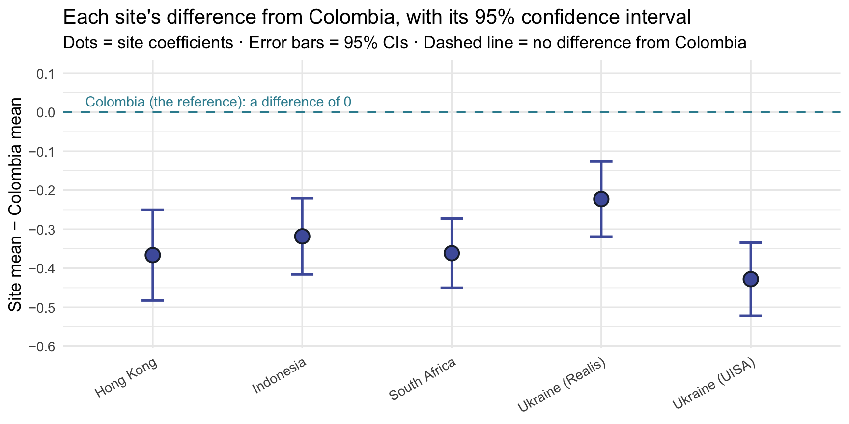
An interval that crossed the dashed line would be a contrast whose 95% CI includes 0 (in test terms, \(|t_\text{obs}| < t^*\) and p > .05). None does here. Keep the two kinds of test apart:
- Each site row tests one comparison: does that site’s mean differ from Colombia’s? Five rows, five separate tests. These are M09’s contrasts, every group compared with the reference, and with five of them, M09’s familywise caution applies.
- The omnibus F from Activity 4.3 tests one joint question: are all six site means equal? It can tell you that some sites differ, but not which ones.
The a-ha moment
The same lm() syntax can handle continuous and categorical predictors, and many continuous outcomes. The core code may stay almost unchanged; what changes is the scientific question, the coefficient interpretation, and whether the linear model’s assumptions are reasonable (M12’s topic).
That single insight is why M11 — multiple regression — is a small extension rather than a totally new framework. Once you’ve fit the regressions on this page, you’ve already done much of what M11 will ask you to do, just on a smaller scale.
Why fit these as regressions at all, if the t-test and ANOVA give the same numbers? Because the linear model keeps going where those tests stop. A two-sample t-test and a one-way ANOVA each answer one fixed question: do these groups’ means differ? Inside a linear model, the same group comparison can share the model with other predictors: adjust a treatment comparison for baseline scores (M11’s first step), mix continuous and categorical predictors, or let an effect depend on another variable. The linear model is also the foundation for more advanced models, such as models for clustered data like participants within sites, or for binary and count outcomes. Learning to read group differences as regression coefficients now is what makes those models a next step rather than a fresh start.
Quick Check
Answer each question — you’ll see green (correct) or pink (incorrect) feedback as you type.
1. True or false: in a regression with one binary predictor, the slope equals the difference between the two group means.
2. You fit lm(t1_benevolence ~ site), where site has 6 levels. How many dummy predictors does R create, and what is the intercept?
3. In Activity 4.3 you fit lm(t1_benevolence ~ site) and also ran anova() on it. How do the two relate?
4. When you fit lm(t2_benevolence ~ treat), the coefficient on treatTreatment is positive. What does the sign mean?
5. In lm(t1_benevolence ~ site), how is the statistic in each site row of tidy() computed?
6. True or false: all five site rows in lm(t1_benevolence ~ site) use the same critical value, \(t^*\).
7. The F-statistic from glance() and the p-value in the siteHong Kong row answer different questions. Which pairing is right?
8. The 95% CI for the siteIndonesia coefficient lies entirely below 0. What can you conclude from that row alone?
9. True or false: the site rows have different standard errors because the sites have different numbers of participants, even though the model uses one residual SD for all of them.
Four things to carry into lecture
- One code pattern, three kinds of predictor. lm() fit every model on this page, and tidy() + glance() read each one; only the kind of predictor on the right of the
~changed, and with it how you read the coefficients. - Every coefficient’s inference is the same recipe. The CI is estimate ± \(t^*\) × SE, \(t_\text{obs}\) is estimate ÷ SE, and the p-value is the two-tailed area beyond \(t_\text{obs}\) — you rebuilt all three by hand for a continuous slope (Activity 3.2) and for five site contrasts at once (Activity 4.4).
- The t-test and the ANOVA live inside lm(). The standard two-sample t is the binary-predictor regression, and the one-way ANOVA is the multi-category regression — same statistics, same df, same p-values, to the decimal.
- With a single categorical predictor, the model reproduces the group means exactly. Computing the means before fitting (Activities 4.1 and 4.3) is the habit that lets you check any single-predictor categorical regression against numbers you already know.
Monday’s lecture builds on these steps, and M11 adds a second predictor to the same lm() call.