Model Assumptions, Diagnostics, and Remediation
Pre-Study · Module 12 · Fri Nov 13
Welcome to the M12 pre-study, the last pre-study of PSY 652. The M12 Module asked whether the site-adjusted model’s answer, a treatment effect of about 0.50 benevolence points, can be trusted, and built a diagnostic for each assumption behind it. Here you build those diagnostics yourself, on the same model, before Monday.
How this page is organized
- Warm-up: refit the model with site, and meet the columns every diagnostic is built from.
- Three short videos, each followed by two or three practice activities and a short Quick Check.
- If this check had failed notes, after the last activity for each assumption, link to the Module section that shows the remedy. Some of our checks look very good; others reveal limitations whose importance depends on what we want to infer.
- Wrap-up: check_model()’s one-figure summary, matched to the plots you built.
Every code activity uses a three-tab panel:
- ✍️ Your Code — the starter with blanks for you to fill in
- 💡 Hint — a nudge in the right direction
- 👀 Spoiler — the full working code if you get stuck
The analysis tibble (n = 3,965) is already loaded, with centered baseline benevolence, t1_benevolence.c, computed.
Warm-up — refit the model you’re about to diagnose
Three quick steps before the first video: refit the model this page diagnoses, look at each participant’s fitted value and residual, and meet the other columns augment() adds.
Refit the model with site
Refit M11’s model with site: the outcome regressed on centered baseline benevolence, treatment, and site.
Your task: fill three blanks — the outcome, the centered baseline-benevolence predictor, and the site predictor.
The outcome is the 2-week follow-up benevolence score. The centered baseline-benevolence column was pre-computed in the setup chunk — its name ends in .c. Site is the study-site variable (six sites in five countries), just called site.
You should see eight rows — the intercept, the slope for centered baseline benevolence, the treat slope, and five site dummies. The treat coefficient is about 0.500, exactly what M11 reported. The model with site is now fit and stored in m2.
Look at each participant’s fitted value and residual
Every diagnostic on this page is built from augment(), the broom function you used in M10 and M11. It returns your data with the model’s results attached, one row per participant. Two of its columns matter most:
- .fitted is the fitted value, \(\hat{y}_i\): the model’s prediction for that participant, given their baseline benevolence, treatment group, and site.
- .resid is the residual, \(y_i - \hat{y}_i\): how far that participant’s observed follow-up score sits from the prediction.
Your task: fill two blanks — the function that attaches the model’s results to the data, and the column to subtract from the observed score so you can rebuild the residual yourself.
The function is the broom verb that adds fitted values and residuals to the data: augment(). A residual is the observed score minus the model’s prediction, and the prediction lives in the .fitted column.
Each row is one participant. Read across a row: t2_benevolence is what that person reported at follow-up, .fitted is what the model predicted for them, and .resid is the gap between the two. Your observed_minus_fitted column matches .resid in every row, because that’s all a residual is. A positive residual means the person scored higher than the model predicted; a negative one means lower. (augment() attaches four more columns, which the last step of this warm-up lays out in one table.)
Why residuals are at the center of M12
A residual is the part of a participant’s score that the model didn’t predict. That makes residuals the raw material for two jobs.
Judging how well the model fits. The fit summaries from M10 and M11 are built from the residuals. The residual standard error, \(\hat{\sigma}\) (0.81 here), our estimate of the errors’ standard deviation, is the typical size of the gap between an observed score and its prediction, in benevolence points. And \(R^2\) (.40 here) compares how spread out the residuals are with how spread out the outcome is: the smaller the residuals relative to the outcome’s own variation, the closer \(R^2\) gets to 1.
Checking the assumptions. Linearity, normality, and equal variance are statements about the model’s errors: the gaps between each person’s score and the true population regression line. You never see the errors, because you never know the true line. The residuals are your estimates of them, so you check those assumptions by checking the residuals. If the model describes the data well, the residuals should look like patternless scatter:
- averaging about zero at every fitted value (linearity, Video 1);
- roughly bell-shaped (normality, Video 2);
- about equally spread out across the whole fitted range (equal variance, Video 2).
A pattern left in the residuals is something the model missed. Video 3 then turns to single participants, asking whether anyone pairs a large residual with unusual predictor values in a way that pulls the fit.
Every column augment() adds
augment() attaches six columns in all, each starting with a dot. Run the cell to see them beside the model’s four variables, one row per participant:
You don’t need to learn them all now. Treat this table as a reference, and come back to it when an activity uses a column. In the formulas, \(k\) is the number of slopes (7 here: baseline benevolence, treatment, and five site columns) and \(n\) = 3,965.
| Column | What it is | How it’s computed | Rule of thumb | Where you use it |
|---|---|---|---|---|
| .fitted | The model’s prediction for this participant, \(\hat{y}_i\) | Plug the participant’s baseline benevolence, treatment group, and site into the fitted equation | — | Warm-up; Activities 1.1, 1.2, 2.2 |
| .resid | The residual: how far the observed score sits from the prediction | Observed minus fitted, \(y_i - \hat{y}_i\) | Judged in plots, not one at a time | Warm-up; Activities 1.1, 1.2 |
| .std.resid | The standardized residual, \(r_i\): the residual on a common scale | \(r_i = (y_i - \hat{y}_i) / (\hat{\sigma}\sqrt{1 - h_{ii}})\), where \(\hat{\sigma}\) is the residual standard error and \(h_{ii}\) is the leverage in the next row | Beyond ±2 is unusual; about 5% of well-behaved data land there (4.9% of ours) | Activities 2.1, 2.2, 3.1, 3.2 |
| .hat | Leverage, \(h_{ii}\): how unusual the participant’s predictor values are | From the predictor values alone; the outcome plays no part. Always averages \((k + 1)/n\), here 0.0020 | High above \(2(k + 1)/n\), twice the average: 0.0040 here | Activities 3.1, 3.2 |
| .cooksd | Cook’s distance: how much all the fitted values would shift if this participant were dropped | Combines the two rows above: \(\dfrac{r_i^2}{k + 1} \times \dfrac{h_{ii}}{1 - h_{ii}}\) | Above 1: clearly worth investigating. Above \(4/n\) (0.0010 here): a sensitive screening heuristic, not a pass/fail threshold | Activities 3.1, 3.2 |
| .sigma | The residual standard error the model would have without this participant | Refit the model without them | — | Not used in M12 |
Cook’s distance multiplies a residual term by a leverage term, so it is largest when a participant has both a large standardized residual and unusual predictor values, though a big enough value of either one alone can also make it large. Video 1’s residual–fitted plot puts .fitted on the x-axis and .resid on the y-axis, one point per participant. The rest of this page diagnoses m2 through these columns, starting with Video 1.
Video 1 — The Five Assumptions and the Linearity Check
Video looks blurry? Click the gear icon at the lower right of the player and set Quality to 1080p, or the highest option offered.
What to listen for:
- Two assumptions about the study’s design come first — validity and representativeness — evaluated from how the study was designed and measured, not from diagnostic plots
- Then five statistical assumptions: Linearity, Independence, Normality, Equal variance, plus Additivity (LINE is a memory aid, not a ranking). Four are checked through the residuals or, for additivity, by comparing models; independence is judged mainly from the design. Also, which two of them M10 and M11 already touched
- The model under diagnosis is the warm-up’s model with site; its treatment estimate, 0.500 (95% CI [0.449, 0.550]), is the answer M12 asks how far to trust
- The residual–fitted plot is the post-fit diagnostic for linearity — predicted values on the x-axis, residuals on the y-axis
- The bounded-outcome wedge: a downward-slanting edge along the top of the cloud is a mechanical consequence of the 1–5 bounds, not a linearity violation
- The LOESS smoother — not the point cloud — is the part you actually read for linearity
- What okay and violated look like, in simulated data: a smoother that runs flat along zero, and one that bends into a U because the model is missing a curved term
- To look at one predictor at a time, the Module builds an added-variable plot, whose slope is exactly that predictor’s coefficient (for curvature in one predictor, the standard check is a component-plus-residual plot)
Activity 1.1 — Build the residual–fitted plot
The standard linearity diagnostic puts \(\hat{y}_i\) on the x-axis and the residual (\(y_i - \hat{y}_i\)) on the y-axis. Use augment(), as in the warm-up, to attach fitted values and residuals, then plot with a horizontal reference line at zero and a LOESS smoother on top.
Your task: fill three blanks — the fitted-value column, the residual column, and the smoothing method.
augment() attaches several columns to the data; the fitted value is in .fitted and the residual is in .resid. The standard smoother for diagnostic plots is a local regression, which goes by the five-letter name loess. It slides a window along the x-axis and, at each spot, fits a gentle curve to just the nearby points, so it can follow a bend that a single straight line would miss.
You should see a downward-slanting edge along the top of the point cloud — the bounded-outcome wedge — and a rose LOESS smoother that hugs zero through the middle of the fitted range, where most participants sit, and dips a little at both sparse ends. The cloud’s shape comes from the 1–5 bounds; the smoother is the linearity check. The smoother stays close to zero where most of the data are, so the plot shows little evidence of a curved relationship there.
Video 1’s “okay” panel was an unusually calm draw. Even when the model is right, a LOESS smoother wobbles by chance, most of all at the sparse ends: with 300 points and an error SD of 1, it typically strays about 0.2 to 0.3 from zero somewhere. Read a bend as evidence when it is large next to that kind of wobble and the bulk of the points follow it.
Activity 1.2 — Quantify the bounded-outcome wedge
To see the wedge story numerically, split the model’s fitted values into three roughly equal-sized bins (low, middle, high) and summarize the residuals in each: their mean now, and their standard deviation for Video 2. The question for now: does the wedge in the cloud translate into a drift in the conditional means? If the linearity assumption holds, it shouldn’t — every bin’s mean residual should sit near zero no matter how the envelope of possible residuals narrows.
Your task: fill three blanks — the variable to bin (the fitted value), the column to average (the residual), and the function for its spread.
The two columns from augment() are the fitted values (.fitted) and the residual (.resid). You want to bin by the fitted value and average the residual. The standard-deviation function is the two-letter sd().
All three bin means land within a few hundredths of zero — and they don’t step monotonically (the middle bin is actually the highest of the three). The wedge you saw in the cloud is an envelope phenomenon: it narrows the range of possible residuals near the boundaries, but it barely tilts the conditional means, which are exactly what the linearity assumption cares about. (The sd_resid column answers a different question, the equal-variance check; Video 2 comes back to it.) The binned means and the LOESS smoother show little evidence of curvature through the middle of the fitted range. They don’t establish that every predictor’s relationship is correctly specified: a residual–fitted plot is an overall check, and patterns can cancel out when they’re averaged together, which is why Video 3 looks at additivity, and why the Module looks at one predictor at a time.
If this check had failed: a smoother that bends systematically, especially through the middle of the fitted range where most participants sit, would suggest that the model’s predictions are missing a pattern in the data: a curve in one predictor, an interaction, or a floor or ceiling of the scale. The residual–fitted plot can’t say which predictor is responsible, so the next step is a plot for one predictor at a time (the Module’s section Which predictors need a linearity check? builds it). The Module’s section What to do when linearity fails lists the standard remedies, such as a squared term for the predictor responsible for the bend. Polynomial terms and transformations for curved relationships are developed in more advanced courses.
Quick Check
Answer each question — you’ll see green (correct) or pink (incorrect) feedback as you type.
1. When you look at a residual–fitted plot for a model whose outcome is bounded (like a 1–5 score) and many scores sit near the top of the scale, you may notice a clear downward-slanting edge along the top of the point cloud. Which of these is the correct interpretation?
2. True or False: A flat LOESS smoother sitting near zero across the full range of \(\hat{y}\) in the residual–fitted plot is consistent with the linearity assumption being (approximately) satisfied.
Video 2 — Normality and Equal Variance: Reading the Residual Distribution
Video looks blurry? Click the gear icon at the lower right of the player and set Quality to 1080p, or the highest option offered.
What to listen for:
- A histogram of the residuals, with a Normal curve for comparison, is a quick first look at their shape
- The Q–Q plot checks normality of the errors through the residuals — the points should fall along the diagonal, with the tails being the part to read most carefully
- The model with site shows a mild negative skew, consistent with the bounded 1–5 outcome: the lower-tail points droop below the line (a heavier-than-Normal lower tail) while the upper tail stays close to it — the boundedness story appearing in the Q–Q plot just as it did in the residual–fitted cloud
- The Central Limit Theorem does a lot of the work at large n: Normality of the errors matters far less than it might seem for coefficient inference, though it still matters for predicting one person’s score
- The scale–location plot (\(\sqrt{|\text{standardized residual}|}\) vs \(\hat{y}\)) checks equal variance — a flat smoother is consistent with homoscedasticity (constant variance)
- A robust-SE sensitivity analysis shows whether the unequal spread materially changes the coefficient inference: for the treatment effect here, the standard error moves by less than 1%
Activity 2.1 — Build the Q–Q plot
The standard normality diagnostic plots the standardized residuals against theoretical Normal quantiles. stat_qq() draws the points; stat_qq_line() draws the reference diagonal.
Your task: fill two blanks — the augment() column to use as the sample, and the name of the function that draws the reference line.
The standardized residual column from augment() is .std.resid. The line-drawing function is stat_qq_line() — same prefix as the points, with _line appended.
The points hug the diagonal across the middle, and the tails tell an asymmetric story: the lower-left points droop below the line (the left tail is heavier than a Normal’s — the occasional participant whose follow-up score lands far below a prediction near the top of the scale), while the upper-right points stay close to the line, drifting slightly above it only at the very end. This mild negative skew is consistent with the bounded 1–5 outcome, with predictions concentrated nearer the ceiling than the floor. At n = 3,965, it matters very little for the coefficients — the CLT delivers approximately Normal sampling distributions for the coefficients under mild conditions (one is that no coefficient rests on just a handful of participants).
If this check had failed: heavy tails or strong skew matter most in a modest sample, or when the model’s job is predicting individuals. For those cases, the Module’s remedies (bootstrap CIs, robust regression, and other kinds of models) are in the Going further box on what to do when normality fails, just below When does the normality assumption actually matter?
Activity 2.2 — Build the scale–location plot
The equal-variance diagnostic plots \(\sqrt{|\text{standardized residual}|}\) against \(\hat{y}\). A flat LOESS smoother is consistent with constant residual variance across the fitted range.
Your task: fill two blanks — the transformation applied to the standardized residual, and the smoothing method.
The abs() part is already filled in; the blank is R’s square-root function, sqrt(). The smoother is the same local regression as in Activity 1.1, loess.
The rose LOESS smoother trends slightly downward across the fitted range — the typical residual magnitude is mildly smaller at high \(\hat{y}\). That fits the bounded-outcome story, now expressed as a variance pattern: the ceiling of the 1–5 scale squeezes how far most residuals can stray at high predicted T2. The smoother’s downward drift is small in absolute terms. (The Module’s robust-SE check shows that the treatment effect’s standard error barely moves, partly because the two randomized arms are close to equal in size, while the other coefficients’ standard errors move more, in both directions.)
Now look back at the sd_resid column of Activity 1.2’s table. The residual SD declines modestly from the low-\(\hat{y}\) bin to the high-\(\hat{y}\) bin — consistent with the ceiling squeeze, and the same gentle downward drift the scale–location smoother shows. The drop is small (a few hundredths of a benevolence point across the full range). Equal variance is a reasonable approximation here. The small remaining heteroscedasticity is consistent with the 1–5 bounds, and the Module’s robust-SE comparison confirms that the usual SE for the treatment effect from lm() barely changes.
If this check had failed: the Module’s worked robust-SE example shows the most practical fix on this same model. Robust standard errors keep the coefficients unchanged and recompute their standard errors without assuming equal variance. The section just above it, What to do when equal-variance fails, lists the other options. Robust SEs repair the coefficients’ standard errors, not the model: they don’t help prediction intervals for individuals, and a large gap between the robust and classical SEs is a cue to look again at the model itself.
Quick Check
Answer each question — you’ll see green (correct) or pink (incorrect) feedback as you type.
1. In the Q–Q plot for the model with site, the lower-left points droop below the reference line while the upper tail stays close to it. What does that pattern indicate?
2. True or False: At a sample size of n = 3,965, the mild negative skew in the model’s residuals will substantially distort the coefficient confidence intervals from lm().
Video 3 — Influence, Overlap, Additivity, and When Violations Matter
Video looks blurry? Click the gear icon at the lower right of the player and set Quality to 1080p, or the highest option offered.
What to listen for:
- Leverage (\(h_{ii}\), the hat value) measures how unusual an observation’s predictor profile is — a property of X alone. A common flag for high leverage is twice the average, \(2(k + 1)/n\): about 0.004 here
- Cook’s distance combines leverage with residual size to measure each observation’s total effect on the fitted values
- A simulated small study shows what influence looks like: in that study, a large residual at ordinary leverage, or high leverage on the trend, moves the fitted line little, while the two together swing it
- Multicollinearity is about predictors’ relationships with each other — not about residuals
- VIF (variance inflation factor) is the standard diagnostic; performance::check_collinearity() reports it for every predictor in one call
- Additivity, the fifth assumption: in an additive model, each predictor’s slope or contrast is the same across values of the other predictors, so the model draws parallel lines
- A check that lets the treatment effect vary with baseline benevolence finds non-parallel lines — a larger effect at lower baseline benevolence: moderation, compression from the bounded scale, or both. These data don’t cleanly separate those explanations: a linear model on the 1–5 scale can’t tell them apart (PSY 653 develops moderation in full)
- For deciding when a violation matters: distinguish bias from inefficiency, attend to sample size, consider your inferential goal, and when the judgment is close, run it both ways
Activity 3.1 — Build the residuals-vs-leverage plot
augment() returns Cook’s distance (.cooksd) and leverage (.hat) as columns. Use them directly to build a residuals-vs-leverage plot — leverage on the x-axis, standardized residual on the y-axis, and color points by their Cook’s distance so the influential cases pop out.
Your task: fill three blanks — the leverage column, the standardized-residual column, and the Cook’s-distance column.
augment() prefixes every diagnostic column with a leading dot. Leverage is .hat, the standardized residual is .std.resid, and Cook’s distance is .cooksd.
Look at the x-axis numbers first: every leverage value is tiny (the axis tops out below 0.005), but ggplot zooms the axis in, so the points fill the plot anyway. The separate group of points on the right is everyone from Hong Kong, the smallest site (323 participants). The model estimates each site’s average from that site’s own participants, so in a small site each person counts for more: every Hong Kong participant has higher leverage than anyone from the other five sites, though still tiny in absolute terms. By the warm-up table’s rule of thumb (more than twice the average leverage, 0.0040 here), 25 of them count as high leverage: the Hong Kong participants whose baseline benevolence sits near one end of the scale. They cross the line only barely, and only next to an average that is itself tiny, and none has a Cook’s distance above 0.005: unusual predictor values alone don’t make a participant influential. The few points out at large negative residuals (beyond −4) sit at ordinary leverage, well left of the flag line. No single observation comes anywhere near the classic Cook’s distance threshold of 1.0. With n = 3,965, no individual participant is in a position to dominate the fit.
Activity 3.2 — Identify the most influential observations
When the residuals-vs-leverage plot does flag points, the substantive next step is to look at them directly. Run this code: it sorts by Cook’s distance, largest first, and prints the top five rows along with each participant’s predictor values.
The top five Cook’s distances are all well below 0.1 — the largest is about 0.0073, far below the classic \(D > 1\) threshold. No observation appears strongly influential in this model. The sensitive \(D > 4/n\) screen (≈ 0.0010 here) does flag a few percent of observations in this dataset. That doesn’t mean those participants are problematically influential: \(4/n\) is a screening heuristic, not a pass/fail threshold, and here even the largest Cook’s distances are very small. When a future model of yours flags genuinely influential points, you’d use this same arrangement to inspect them, then fit the model with and without them to test robustness.
If this check had failed: the Module’s section What to do when influential observations are present walks through those steps, including what to look for when you investigate the flagged observations and when robust regression is worth considering.
Activity 3.3 — Check multicollinearity with VIF
The standard multicollinearity diagnostic is the variance inflation factor. performance::check_collinearity() reports it for every predictor in the model in a single call — the same function the Module used. For a predictor with a single coefficient, a VIF of 1 means the other predictors don’t linearly predict it at all, and values near 1 mean very little collinearity; values above 5 or 10 are conventionally flagged. Run it:
Every VIF is close to 1 — the largest is about 1.02, well below the 5–10 warning thresholds. There’s essentially no multicollinearity in the model with site, which is exactly what we’d expect: random assignment makes treatment nearly uncorrelated with baseline benevolence and with site, and site and baseline benevolence are only weakly correlated. (performance::check_collinearity() reports one term-level generalized VIF for a factor predictor like site — a single number covering all five site dummies at once — and the same reading applies: a value near 1 means almost no overlap with the other predictors.) The output also prints a 95% CI for each VIF; read the VIF column itself. (The version of performance in this page’s sandbox computes that interval with an older method that can show an enormous upper end for a VIF near 1, as in treat’s row. Current versions, like the one you’ll install in RStudio, don’t.)
If this check had failed: when a predictor you need to interpret has a high VIF (5 and 10 are the conventional flags) and its confidence interval is too wide to answer your question, open the Going further box on remedies at the end of the Module’s VIF section. To see the remedies for every check in one place, the Module’s remediation toolkit summary gives each problem, its diagnostic, and the first fix to reach for in a single table.
Quick Check
Answer each question — you’ll see green (correct) or pink (incorrect) feedback as you type.
1. Leverage (\(h_{ii}\), the hat value) and Cook’s distance both help flag potentially influential observations, but they measure different things. What does Cook’s distance take into account that leverage doesn’t?
2. True or False: A bias-inducing assumption violation (like a missing interaction or omitted confounder) can be fixed by collecting a larger sample, because the CLT will take care of it.
Wrap-up — all the checks in one call
You’ve now built every diagnostic plot for the model with site yourself. The performance package’s check_model(), which the Module introduced in Parts 5 and 8, draws them all in a single call. Here is its output for our model. There’s nothing to run this time: the figure was drawn when this page was built, because check_model() needs the see package and a full-size plot pane. You’ll run it yourself in the lab, in RStudio.
m2 |>
  performance::check_model()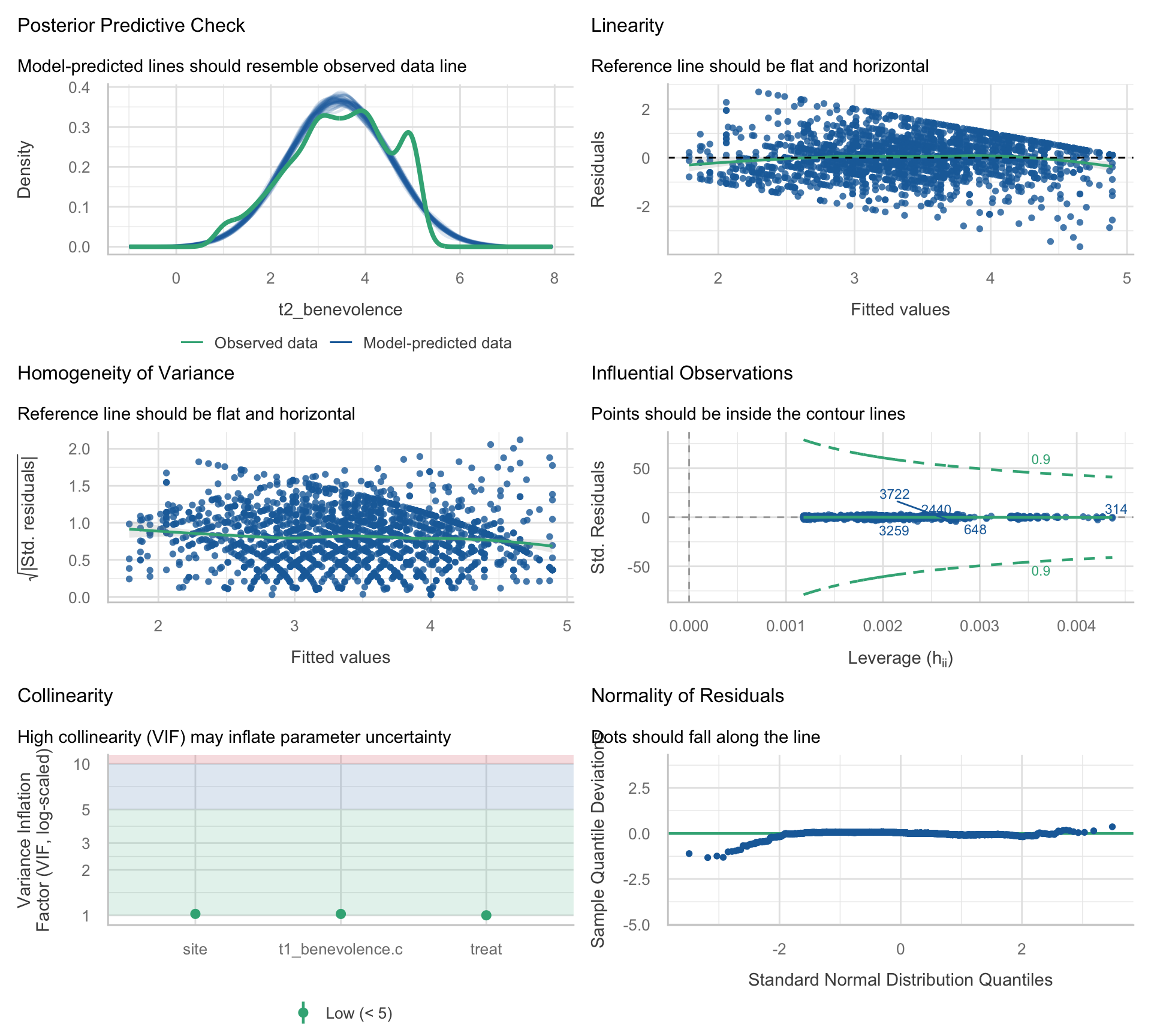
Match each panel to the plot you built
Five of the six panels repeat a check you built by hand. For each panel, pick the activity where you built the same check:
- Posterior Predictive Check (top left):
- Linearity (top right):
- Homogeneity of Variance (middle left):
- Influential Observations (middle right):
- Collinearity (bottom left):
- Normality of Residuals (bottom right):
What the summary adds
The one check you didn’t build, the posterior predictive check (the package’s name for it), compares the real outcome with outcomes simulated from the fitted model. Each thin blue curve is one simulated dataset: every participant’s fitted value plus a Normal error with the model’s residual SD. The green curve is the real T2 benevolence scores. If the model reproduced the outcome’s shape, the green curve would sit among the blue ones. Here it doesn’t. The 10.8% of participants who score exactly 5 make a spike near 5 that none of the simulations has, and the simulated curves run below 1 and past 5, scores no participant could report. That’s the bounded-outcome story from Videos 1 and 2, seen this time from the outcome’s side. It matters little for the treatment effect, and more for predicting one participant’s score.
The other five panels agree with what you found by hand: little sign of curvature, residual spread close to constant apart from the mild squeeze near the ceiling, no influential participants, VIFs near 1, and approximately Normal residuals apart from the heavier lower tail. Two details look different from your versions:
- The normality panel is detrended, so its dots should follow a flat line at zero instead of a diagonal.
- The influence panel’s dashed curves are check_model()’s Cook’s-distance screening contours; points outside them would be flagged as influential. The few labeled points have the largest Cook’s distances among the dots drawn, which here are a random sample, so they need not be the five largest overall. A label isn’t a flag.
The Module explains both in Part 5.
The four diagnostic questions
Every check on this page answers one of four questions:
| Question | Main tools | Where you practiced it |
|---|---|---|
| Does the model capture the average relationship? | Residual–fitted plot; a check of additivity | Activities 1.1–1.2 (additivity: Video 3) |
| Are the errors’ shape and spread acceptable for what we want to conclude? | Q–Q plot; scale–location plot | Activities 2.1–2.2 (and Activity 1.2’s SD column) |
| Is any single observation pulling the fit too much? | Leverage; Cook’s distance | Activities 3.1–3.2 |
| Do the predictors overlap too much to interpret each coefficient precisely? | Variance inflation factor (VIF) | Activity 3.3 |
Independence of errors isn’t on this list, because it is judged mainly from the study design (the Module’s Part 1).
Four things to carry into lecture
- The diagnostic plots are statistics about the model, not the world. Q–Q plots almost never look perfectly straight; the right question is rarely “is this violated” and almost always “is this violation large enough — given my sample size and inferential goal — to change what I should report.”
- Read the smoother, not the cloud. For both the residual–fitted and scale–location plots, the LOESS smoother is the part that answers the diagnostic question. A wedge or funnel in the cloud often comes from a bounded outcome — a feature of the 1–5 scale rather than a mis-specified mean.
- Distinguish bias from inefficiency. Bias-inducing violations (linearity, additivity, omitted confounders) need structural fixes, and no sample size repairs them. Influence sits between the two and is checked in the sample you have. Among the inefficiency-type problems, non-Normal errors are forgiven at large n; heteroscedasticity calls for an SE-level check (robust SEs or the bootstrap) at any n, because a large sample doesn’t fix the classical SEs; modest multicollinearity mostly widens CIs.
- Non-parallel lines mean the treatment contrast differs across the other predictor — moderation, compression from the bounded scale, or both. For REACH, these data don’t cleanly separate those explanations: a linear model on the 1–5 scale can’t tell them apart. When the difference is substantive, the additive treatment coefficient can still serve as an overall summary of a contrast that varies across baseline benevolence. PSY 653 develops moderation in full.