The Logic of NHST

Pre-Study · Module 8 · Fri Oct 2

Welcome to the M08 pre-study. The Module gave you the textbook treatment of NHST — the null hypothesis, the bootstrap null distribution, the p-value, the test statistic, and the parametric one-sample t-test. This pre-study is where those pieces click into place through hands-on practice.

How this page is organized

Four short videos drive home the Module’s hardest conceptual moves. After Video 1 you’ll write hypotheses and pick benchmarks. After Video 2 you’ll build a null distribution and compute a p-value the right way. After Video 3 you’ll see the bootstrap standardized into the language of test statistics (\(t_\text{obs}\)). After Video 4 you’ll run the parametric one-sample t-test and confirm it agrees with the bootstrap. The page closes with a short self-test on the most consequential p-value misconceptions.

Every code activity uses a three-tab panel:

• ✍️ Your Code — the starter with blanks for you to fill in
• 💡 Hint — a nudge in the right direction
• 👀 Spoiler — the full working code if you get stuck

Work through the ✍️ tab first. Only open 💡 or 👀 after you’ve tried it yourself — struggling a little is how this stuff sticks. Plan on about 60 minutes for the whole page.

---

The college_mobility dataset (and our canonical sample)

The pre-study uses the same dataset as the M07 Module: 2,199 U.S. colleges with median earnings at age 34 for the cohort of students who attended each institution (Chetty et al., 2017). The dataset is already loaded into your sandbox under the name college_mobility.

college_mobility · 2,199 observations · 2 variables

• name character — Institution name
• k_median numeric — Median individual earnings, in 2014 US dollars, among the college’s former students

Because we’re treating these 2,199 colleges as our reference population, we can compute its mean exactly: $36,929. The repeated-sampling behavior of every procedure you run can be checked against that number — a luxury real research never has.¹

Full codebook for college_mobility — values, levels, missingness, and how the file was prepared.

We’re also re-using the exact 50-college sample you drew in M07’s PS1 video chain, so the numbers in the videos match what you saw last week. The setup chunk above already built it for you under the name my_sample, alongside its derived constants (xbar, s, n, SE) and our chosen benchmark (mu0 = $32,000).

---

Video 1 — Where Does μ₀ Come From?

What to listen for:

• M07 left us with a 95% bootstrap CI from one sample of 50 colleges: roughly $34,100 to $39,900
• Testing requires something the CI doesn’t: a specific benchmark to compare against — that’s \(\mu_0\)
• Three candidate benchmarks for our college-vs-no-college comparison: $11,500 (Chetty), $12,000 (poverty line), $32,000 (NCES)
• The NCES benchmark wins because it has a clean interpretation: matched to our cohort’s age band, and restricted to full-time, year-round workers
• We acknowledge the honest trade-off: NCES narrows the comparison to “the typical full-time, year-round worker with a high school diploma and no college”
• \(H_0: \mu = \$32{,}000\) and \(H_a: \mu \neq \$32{,}000\) — note the two-sided default
• The decision threshold \(\alpha = .05\), pre-specified before looking at the data — the cutoff that turns the (continuous) p-value into a binary reject / fail-to-reject decision

Activity 1.1 — Write \(H_0\) and \(H_a\) for the college-mobility test

In the Module, we wrote the hypotheses for our college-mobility test in symbols. Let’s make sure the structure sticks.

Your task: fill the two blanks — the value \(\mu_0\) that goes in \(H_0\), and the comparison operator that goes in \(H_a\) for a two-sided test.

✍️ Your Code

💡 Hint

The benchmark we picked from NCES is in 2015 dollars. The two-sided alternative says “different from \(\mu_0\) in either direction” — what’s R’s symbol for “not equal”?

👀 Spoiler

In our notation: \(H_0: \mu = \$32{,}000\) and \(H_a: \mu \neq \$32{,}000\). The two-sided default holds even when our substantive question is directional — we’d want to know about a surprising deviation in either direction.

Activity 1.2 — Evaluate three candidate \(\mu_0\) values

Imagine a different scenario. A clinical psychologist is testing whether their new brief-CBT intervention reduces post-treatment depression scores. They’re considering three candidate values for \(\mu_0\):

• (A) Zero — on the intuition that “zero means no effect”
• (B) The clinic’s documented mean post-treatment PHQ-9 score (10.4) among patients who received treatment as usual over the past three years
• (C) A round number from the literature — say 12 — picked because it’s between mild (10) and moderate (15) depression

For a one-sample test of post-treatment PHQ-9 against \(\mu_0\), which of these makes the best \(\mu_0\), and why?

(A) Zero — since zero should mean the intervention had no effect(C) A literature round number — gives a publishable comparison pointAny of them is fine — the choice doesn’t affect the test(B) The clinic’s own treatment-as-usual mean — anchored, defensible, and answers the substantive question

Tip👀 Open after you’ve chosen your answer

(A) tests the wrong thing. On the PHQ-9 (0 to 27), a score of 0 means no symptoms at all, so \(\mu_0 = 0\) asks whether the average treated patient is completely symptom-free. Any real clinical sample rejects that immediately — and learns nothing about whether the intervention helped. Zero means “no effect” only when the quantity being tested is itself a change or a difference. Here it is a raw score, so zero is just the floor of the scale.

(C) answers no one’s question. Twelve is a round number between two cutoffs; nobody is asking whether the average patient lands there.

(B) is the best choice. It asks whether patients did better than under the clinic’s usual care — the question stakeholders actually want answered, anchored in real data. One caveat: it is a historical benchmark, so it treats 10.4 as known exactly and assumes past and present patients are comparable. A concurrent comparison group would be stronger.

The rule to carry forward: a good \(\mu_0\) is a real comparison someone in your field cares about, with a source you can point to — and when the outcome is a raw score, that comparison is almost never zero.

Quick Check

Answer each question — you’ll see green (correct) or pink (incorrect) feedback as you type.

1. A 250-college sample produced a sample mean of $37,187. We want to test whether mean college-attendee earnings differ from $32,000. Which is the correct null hypothesis?

H₀: μ = $32,000H₀: x̄ = $37,187H₀: x̄ = $32,000H₀: μ = $37,187

2. The p-value is computed under \(H_0\) rather than \(H_a\). Why?

Tradition — Fisher proposed it that wayOnly H₀, together with the model’s assumptions, pins down a distribution we can compute probabilities fromBecause Hₐ is always wrongBecause the null is more likely to be true

3. Our substantive research question is directional (“do college attendees earn more?”), but our test uses \(H_a: \mu \neq \$32{,}000\). Why?

It’s a math error in the ModuleTwo-sided is required by APA styleThe two-sided test is the conservative default — we’d want to know about a surprising result in either directionBecause we don’t know which direction the effect goes

4. True or false: when picking a \(\mu_0\) value, the analyst’s choice is mostly a substantive judgment about which comparison answers a meaningful research question, not a mechanical step.

TRUEFALSE

---

Video 2 — Build a Null World; Read the p-value

What to listen for:

• The null sampling distribution is a “what if \(H_0\) were true” thought experiment
• The bootstrap-shift mechanic — resample, then add \((\mu_0 - \bar{x})\) to recenter the distribution at \(\mu_0\)
• The p-value is the proportion of null-world resamples at least as extreme as our observed mean
• A small but principled correction: even when zero resamples are extreme, the underlying tail probability isn’t literally zero. Use \((B+1)\) in the denominator and the \(({\rm extremes}+1)\) in the numerator
• Decision: \(p \approx .001\) → reject \(H_0\) at \(\alpha = .05\)

Before you start: switching to a smaller sample, \(n = 25\)

The video you just watched ran the test on the n = 50 sample you first met in M07’s PS1. For the hands-on activities from here on, you’ll switch to a new sample of 25 colleges, drawn fresh from the same population — and you’ll stay on it through the end of the page, even though Videos 3 and 4 keep narrating the \(n = 50\) sample.

Why switch? Sample size controls a test’s power to detect an effect: the smaller the sample, the wider the null distribution, and the more sampling noise stands between you and a rejection. The Module’s worked example used \(n = 250\); the videos use \(n = 50\). Working at \(n = 25\) lets you see what happens when the sample shrinks further — watch what happens to the p-value, and to the decision.

One caveat. The two samples are different draws, not the same colleges analyzed twice, so this shows what can happen with a smaller sample rather than isolating the effect of \(n\). As it happens, their gaps from \(\mu_0\) are nearly identical ($5,092 at \(n = 50\), $5,108 at \(n = 25\)), but the \(n = 25\) sample is noisier (\(s \approx\) $11,032 at \(n = 50\), $14,803 at \(n = 25\)). Isolating \(n\) cleanly takes many draws at each size — which you’ll do together in Monday’s lecture.

my_sample_25 · 25 observations · seed-4242 draw from college_mobility

The working sample for every hands-on activity from here on — Activities 2.1 through 4.2. Loaded automatically into your sandbox as my_sample_25, with helper constants xbar_25, s_25, n_25, and SE_25 also available. Watch the suffix: the video sample’s constants are still in your sandbox too, under the plain names xbar, s, n, and SE. Typing one of those by mistake won’t raise an error — it will quietly use the \(n = 50\) sample — so from here on, every name you type should end in _25.

The values you’ll find:

• \(\bar{x}\) ≈ $37,108 (mean of within-college medians, in the \(n = 25\) sample)
• \(s\) ≈ $14,803 — noticeably noisier than the \(n = 50\) sample

Nothing to set up — the sample and its constants are already in your sandbox before you touch anything. Run the chunk below only to see them, so the numbers in the activities aren’t abstractions:

Activity 2.1 — Bootstrap and shift (on the \(n = 25\) sample)

You’re about to do exactly what you just watched, step for step — only the input changes, from my_sample to my_sample_25. The mechanics should feel familiar even though the numbers won’t match the video.

Resample with replacement, take each resample’s mean, then add \((\mu_0 - \bar{x})\) to every mean so the distribution centers on the value \(H_0\) claims. That shift is what turns an ordinary bootstrap into a null distribution.

What the shift actually does in the n = 25 sample

This is the one line in M08 that trips people up, so let’s walk it with real numbers before you write it.

Left alone, the bootstrap distribution you are about to build centers itself on your sample mean ($37,108 in the n = 25 sample) — resampling can only echo the data it was handed, so its center lands wherever your sample’s center is. But that’s not the world we want to test. \(H_0\) claims the true mean is $32,000. To ask “how surprising is our result if \(H_0\) were true?” we need that distribution centered on $32,000 instead. So we move it:

\[\mu_0 - \bar{x}_{25} = \$32{,}000 - \$37{,}108 = -\$5{,}108\]

Adding \(-\$5{,}108\) to every resample mean slides the entire distribution down by $5,108, landing it on \(\mu_0\). Note the sign — “add the shift” is standard phrasing, but here the shift is negative, because our sample mean sits above the null value.

Why this is legitimate. Every resample mean moves by the same amount, so the distances between them never change: the center moves, the spread doesn’t. That’s the whole trick. We keep the variability our real data exhibits — which we measured, and trust — and impose only the center \(H_0\) asserts, which is the thing we’re putting on trial. The result is a picture of what sampling noise alone would produce if the null were true.

See it for yourself — here are the actual 5,000 resamples, before and after the shift. These are the very numbers you’re about to generate.

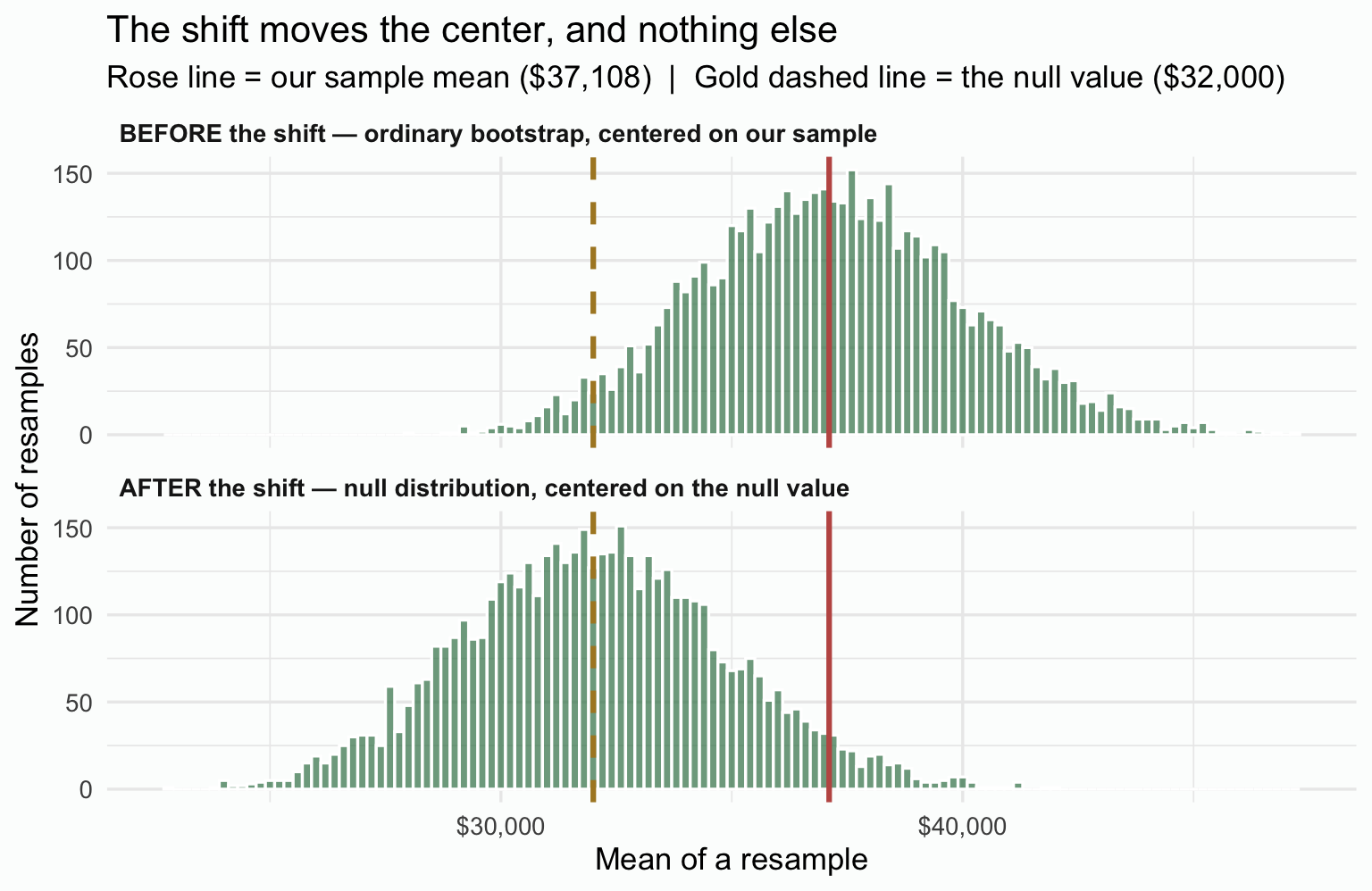
And the same thing as numbers:

	Center (mean of the 5,000 means)	Spread (SD of the 5,000 means)
BEFORE the shift — ordinary bootstrap, centered on our sample	$37,161	$2,856
AFTER the shift — null distribution, centered on the null value	$32,053	$2,856

The center moves by our $5,108; the spread is unchanged. (The centers land a few dollars off $37,108 and $32,000 because 5,000 resamples carry a little simulation noise — run it with a different seed and those last digits wobble.)

Your task: three blanks.

1. n — how many colleges in each resample. A bootstrap resample must be the same size as the original sample, so type 25 — not n, which in your sandbox still holds the video sample’s 50. (That’s what makes each resample a stand-in for a fresh study of the same size.)
2. reps — how many resamples: 5,000, matching the Module.
3. The shift — the gap between the null value and this sample’s mean: mu0 - xbar_25. (Note the 25: we’re on my_sample_25, not the \(n = 50\) sample.)

✍️ Your Code

💡 Hint

• n is the size of each resample — the same size as the sample you drew from, so 25.
• reps is 5,000 (matches the Module).
• The shift is the quantity that moves a resample mean from being centered at \(\bar{x}_{25}\) to being centered at \(\mu_0\) — that is, \(\mu_0\) minus \(\bar{x}_{25}\). In code, mu0 - xbar_25.

👀 Spoiler

The mean of mean_null should come out close to $32,000 — the shift worked.

A note on the spread. This null distribution is wider than the one in the video, for two reasons. The sample is smaller — the SE scales with \(1/\sqrt{n}\), so halving \(n\) alone would widen it by \(\sqrt{2} \approx 1.41\) — and this sample is also more variable. Together they make it about 1.9 times as wide. A wider null means more null-world resamples can reach our observed gap; you’ll see that in the next activity.

Activity 2.2 — Count the extreme resamples

The p-value comes from a count: how many of the 5,000 null-world resamples are at least as far from \(\mu_0\) as our observed sample mean? Before we apply any correction, let’s just count, so the number we get tells us something concrete about the null world.

Two-tailed reminder: “at least as far” means in either direction — a resample mean far below \(\mu_0\) is just as extreme as a resample mean far above. So we use the absolute value: \(|{\rm mean\_null} - \mu_0| \geq |\bar{x}_{25} - \mu_0|\).

Your task: fill the single blank with the observed gap in absolute value (the same \(|\bar{x}_{25} - \mu_0|\) that defines the threshold).

✍️ Your Code

💡 Hint

The observed gap compares your \(n = 25\) sample mean (xbar_25) to your null value (mu0) — the same two quantities you’ve been using all along. Wrap the difference in abs() so the gap is positive whether \(\bar{x}_{25}\) is above or below \(\mu_0\).

👀 Spoiler

You should get 380 — that is, 380 of the 5,000 null-world resamples are at least as far from $32,000 as our observed mean of $37,108 (165 in the left tail, 215 in the right). Compare the Module’s \(n = 250\) example, which got 0, and the videos’ \(n = 50\) example, which got 4.

Dividing by \(B\) gives the naive p-value: \(380 / 5{,}000 = .076\). That’s above \(\alpha = .05\), so the decision is fail to reject \(H_0\). Before reporting it, Activity 2.3 applies one small refinement.

What you just counted, in one picture. Every bar is a slice of the same null distribution you built. The bars shaded rose are the resamples that met the “at least as extreme” test — these are the 380 you counted:

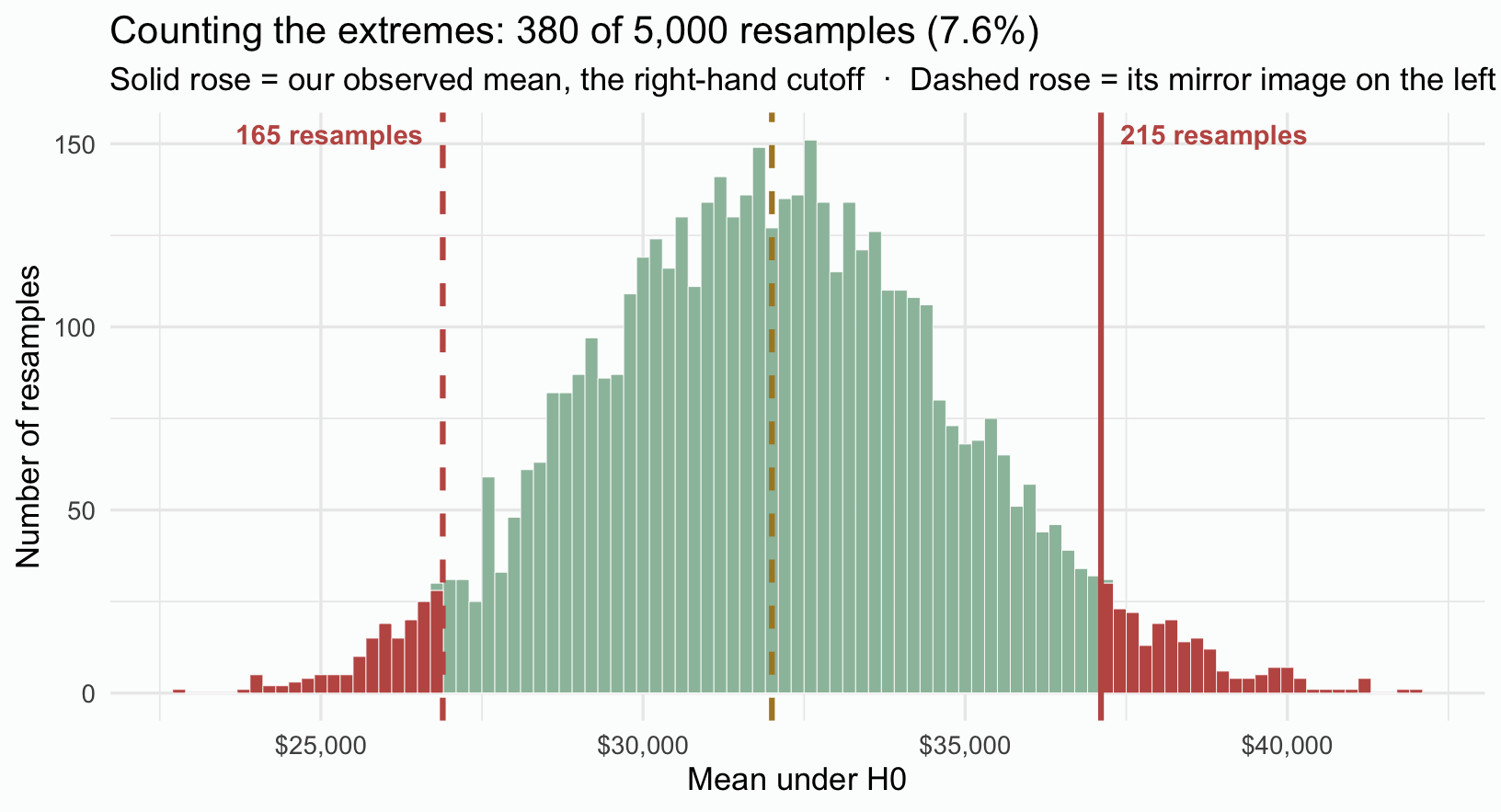
The right-hand cutoff is our observed mean — that’s what “at least as extreme as what we saw” means — and the left-hand cutoff is its mirror image, the same distance below \(\mu_0\). That mirroring is the two-tailed test.

Activity 2.3 — Apply the (B+1) correction

Your p-value came out of a simulation, not a formula — you counted 5,000 randomly generated resamples. An estimate obtained this way, by generating many random draws and counting, is called a Monte Carlo estimate, and it carries a little random wobble: run it again with a different seed and the count shifts slightly.² The Module’s refinement adds 1 to both numerator and denominator:

\[p_{\rm boot} \;=\; \frac{n_{\rm extreme} + 1}{B + 1}\]

The reason in one line: a count of zero extremes doesn’t mean the tail probability is zero — it means you haven’t simulated long enough to see one — so the \(+1\) keeps the reported p-value strictly positive, and applying it always (not just when the count is zero) gives one consistent rule with no special cases.

Here it barely matters: with 380 extremes the p-value moves from .0760 to .0762. It’s still the right form to report.

Two finer points, if you want the justification behind the formula.

Where it’s exact, and where it isn’t. The \((X + 1)/(B + 1)\) form has a formal unbiased estimator derivation for random permutation tests (Phipson & Smyth, 2010), where the observed arrangement of the data is exchangeable with the simulated ones — so the thing you actually observed can legitimately be counted as one more valid draw under \(H_0\). That is what the \(+1\) in the numerator represents. Our procedure is a shifted bootstrap rather than a permutation test, so treat the correction here as a principled, conservative finite-simulation adjustment rather than an exact theoretical guarantee.

Why “conservative” is the right word. The corrected value is always slightly larger than the naive \(X/B\), so it errs toward not rejecting. Given that the whole point of the correction is honesty about what a finite simulation can resolve, erring in the direction of claiming less is the right way to be wrong.

Your task: fill the two blanks — the +1 in each position of the corrected formula.

✍️ Your Code

💡 Hint

It’s quite literally the (B+1) correction — add 1 to the numerator’s count and add 1 to the denominator’s \(B\).

👀 Spoiler

You should get 0.0762. We fail to reject \(H_0\) at \(\alpha = .05\), and report \(p \approx .076\).

The bigger picture. In the videos (\(n = 50\)), the bootstrap p was about .001 — a confident rejection. At \(n = 25\) it is .076, and we can no longer reject. The population hasn’t changed; our power to detect the gap has. Smaller sample → wider null → more resamples reach our observed gap → bigger p.

Activity 2.4 — Plot the null distribution with the observed mean

A picture is worth a thousand words. Visualize the null distribution as a histogram, with the observed sample mean drawn in as a vertical line. The further out our mean sits relative to the width of the null distribution, the smaller the p-value.

Your task: one blank — map the shifted null-world column, mean_null (the one you built in Activity 2.1, centered at \(\mu_0\)), to x. Careful: null_dist also carries the unshifted mean_resample, which would draw the histogram in the wrong place.

✍️ Your Code

💡 Hint

We want to plot the shifted distribution — the one centered at \(\mu_0\). That’s the column we just built in Activity 2.1.

👀 Spoiler

The rose line sits in the right tail, but the null distribution is wide enough that a good share of null-world means reach beyond it: about 7.6% are at least as extreme, in either direction — that’s your p-value. In the \(n = 50\) video the observed mean cleared the tail by a wide margin; this picture is what a non-rejection looks like.

Quick Check

Answer each question — you’ll see green (correct) or pink (incorrect) feedback as you type.

1. What does the null sampling distribution represent?

The actual sampling distribution of the sample meanThe distribution of the populationThe bootstrap distribution from M07What sampling would look like if H₀ were true — a ‘what if’ world

2. When we shift the bootstrap distribution by \((\mu_0 - \bar{x})\), what changes?

Only the center moves; the spread stays the sameBoth the center and the spread moveOnly the spread changesNothing changes — it’s a label change only

3. Why do we use \((B + 1)\) in the denominator (and add 1 in the numerator)?

To make the p-value smallerTo avoid reporting a literal p = 0 — a finite simulation can’t rule out an extreme outcome we just didn’t sampleIt’s how Fisher originally derived the formulaConvention from epidemiology

4. A bootstrap p-value comes out to \(0/5{,}000\) uncorrected (no resamples were as extreme as the observed mean). With the (B+1) correction, what should we report?

p = 0p = .05The corrected estimate is p = 1/5001 ≈ .0002, reported as p < .001p = 1.0

---

Video 3 — Standardizing the Null Distribution

What to listen for:

• Standardization is just a change of ruler — same evidence, expressed in standard-error units instead of dollars
• For each null-world resample mean \(m\), compute \(t = (m - \mu_0)/SE_b\). The shape doesn’t change; the units do.
• The standardized null distribution is centered at ≈ 0 with \(SD = 1\) — by construction (subtracting \(\mu_0\) centers it; dividing by \(SE_b\) rescales it)
• The observed standardized score has a name: \(t_\text{obs}\) — the “observed t-statistic”
• This is the same standardizing move the parametric t-test will use in Video 4

Activity 3.1 — Standardize: how unusual is the gap in \(SE_b\) units?

Reminder: From here on, use the _25 objects: my_sample_25, xbar_25, s_25, n_25, and SE_25.

Video 3 standardized the \(n = 50\) sample; now apply the same three lines to your \(n = 25\) bootstrap, rescaling the dollar gap into standard-error units:

\[ t_\text{obs} \;=\; \frac{\bar{x}_{25} - \mu_0}{SE_b} \]

where \(SE_b\) is the SD of your 5,000 bootstrap resample means. The parametric t-test in Video 4 computes the same statistic, with \(s/\sqrt{n}\) in place of \(SE_b\).

Standardizing divides both sides of the “at least as extreme” comparison by the same positive number, so it can’t change which resamples qualify — your count should match Activity 2.2 exactly. You’ll check that below.

Your task: three blanks. \(SE_b\) is the SD of the resample means — pipe into sd(). The observed score standardizes this sample’s mean, xbar_25 — not xbar, the video sample’s mean. And the per-resample standardization applies the same formula to the shifted column mean_null (not mean_resample).

✍️ Your Code

💡 Hint

For Step 1, the SD of the bootstrap distribution is its standard deviation — that’s just sd(). For Step 2, the observed sample mean for the \(n = 25\) sample is xbar_25 (you’ve been using it throughout V2’s activities). For Step 3, the column inside null_dist that holds the shifted null-world means is mean_null.

👀 Spoiler

Your \(SE_b\) should be about $2,856 and your \(t_\text{obs}\) about 1.79 — your sample mean sits about 1.79 standard errors above \(\mu_0\).

Now confirm the standardized count matches the unstandardized count from Activity 2.2:

The counts match (380 each): standardizing changed the units, not the answer.

Finally, look at where your \(t_\text{obs}\) sits in the standardized null distribution. The histogram below shows your 5,000 standardized null-world means with a rose vertical line marking \(t_\text{obs} \approx 1.79\):

The same evidence, two rulers

Activity 2.2’s dollar-scale count and Activity 3.1’s standardized \(t_\text{obs}\) are the same test in different units, so they must reach the same decision. What standardizing buys you is a universal scale: a \(t_\text{obs}\) of 1.79 has the same interpretation — a distance measured in standard errors — in any study, in a way that “$5,100 above $32,000” does not. Every parametric test uses this scale.

---

Video 4 — The Parametric One-Sample t-Test

What to listen for:

• Every parametric NHST has four ingredients: a point estimate, a null value, a standard error, and a reference distribution
• The parametric SE is \(s/\sqrt{n}\) — a closed-form formula instead of resampling
• The t-distribution at \(df = n - 1\) replaces the bootstrap histogram (smoother, mathematically derived)
• The critical value \(t^*\) defines the rejection region: reject when \(|t_\text{obs}| \geq t^*\)
• infer::t_test() runs the whole test in one call
• Cohen’s d is the effect size — gap divided by \(s\) (the sample SD), not by SE

Activity 4.1 — Run the test with t_test()

Reminder: From here on, use the _25 objects: my_sample_25, xbar_25, s_25, n_25, and SE_25.

Video 4 ran the parametric test on the \(n = 50\) sample; now run it on your 25 colleges. infer::t_test() does the whole test in one call and returns a one-row tibble: the statistic (\(t_\text{obs}\)), its degrees of freedom, the p-value, the alternative, the sample mean (estimate), and the bounds of the 95% CI.

Your task: fill two blanks — the response variable and the null value.

✍️ Your Code

💡 Hint

• Blank 1: the variable in my_sample_25 that holds median earnings — k_median.
• Blank 2: the no-college benchmark — mu0 (already defined as $32,000).

👀 Spoiler

Read off the output:

• statistic ≈ 1.73 — your \(t_\text{obs}\).
• t_df = 24 (\(n - 1\)).
• p_value — p = .097, above \(\alpha = .05\). Fail to reject \(H_0\).
• estimate = $37,108 — the sample mean.
• lower_ci, upper_ci = [$30,998, $43,218] — the parametric 95% CI. It contains \(\mu_0\) = $32,000, which is the CI form of “fail to reject.”

Where does that statistic come from? It’s the same standardized gap you built in Activity 3.1 — the gap divided by a standard error — with one change: the SE comes from a formula, \(s/\sqrt{n}\), instead of from your 5,000 resamples. Rebuild it and check.

Your task: one blank — the denominator of the parametric SE.

✍️ Your Code

💡 Hint

\(\sqrt{n}\), with \(n = 25\) — so sqrt(25), or sqrt(n_25).

👀 Spoiler

Your t_obs_param should match the statistic column exactly. Now compare the two SEs: the formula gives $2,961, against the $2,856 your bootstrap produced in Activity 3.1 — two very different procedures, agreeing to within about 4%. That is the whole difference between the two routes: the same gap and the same null value, but a formula SE instead of a resampled one, and a smooth \(t_{24}\) curve instead of your simulated histogram as the reference distribution. Read against that curve, your \(t_\text{obs}\) falls inside the critical values of \(\pm 2.06\), short of the rejection region — the same fail-to-reject verdict.

Two routes, one answer

You’ve now run the same test on the same 25 colleges two ways:

	Bootstrap (Activities 2.1–3.1)	Parametric t-test (Activity 4.1)
Standard error	\(SE_b\) ≈ $2,856 (SD of resamples)	\(s/\sqrt{n}\) ≈ $2,961
Test statistic	\(t_\text{obs}\) ≈ 1.79	\(t_\text{obs}\) ≈ 1.73
Reference distribution	5,000 null-world resamples	\(t\)-distribution, \(df = 24\)
p-value	\(\approx .076\)	p = .097
Decision at \(\alpha = .05\)	Fail to reject \(H_0\)	Fail to reject \(H_0\)

The two p-values aren’t identical, and shouldn’t be: one counts simulated resamples, the other reads a tail area off a smooth curve. What matters is that two procedures built on different machinery reach the same verdict about the same sample. The bootstrap shows the logic by simulation; the t-test gives the shortcut with a formula. M09 reuses this recipe for two-sample, paired, ANOVA, and chi-square tests — with different SE formulas and reference distributions.

Activity 4.2 — Effect size: Cohen’s d (one-sample form)

The t statistic and p-value tell us whether the gap is surprising under the null — but not how large the gap is in interpretable units. That’s the role of the effect size. Cohen’s d for the one-sample form is the gap divided by the sample SD:

\[d \;=\; \frac{\bar{x} - \mu_0}{s}\]

Notice the divisor: \(s\), not \(SE\). The SE shrinks as \(n\) grows, which inflates \(t_\text{obs}\); \(s\) estimates the population SD and doesn’t systematically shrink, so \(d\) doesn’t grow with sample size the way \(t\) does.

Your task: fill the single blank — the divisor in the Cohen’s d formula.

✍️ Your Code

💡 Hint

The divisor is the sample SD, s_25 (already in your sandbox). For one-sample d, never divide by the SE — that gives you back \(t_\text{obs}\) itself, not Cohen’s d. The two are related by \(t_\text{obs} = d\sqrt{n}\).

👀 Spoiler

You should see \(d \approx\) 0.35 — a small-to-medium effect by Cohen’s conventions (\(d = 0.2\) small, \(0.5\) medium, \(0.8\) large). The effectsize::cohens_d() output adds a 95% CI on \(d\). As the Module insists: always report the CI on d alongside the point estimate — the point estimate alone hides how precisely \(d\) itself was measured.

Notice what just happened. The test said fail to reject — yet \(d \approx 0.35\) says the estimated gap is not trivial. Both are true at once: the gap would be worth caring about if it’s real, and 25 colleges simply aren’t enough to establish that it is. A write-up that said only “p > .05, no effect” would throw that distinction away.

APA-style reporting · your \(n = 25\) result

The Module’s checklist calls for five elements: descriptives, the test statistic with its \(df\), the p-value, a CI on the parameter, and an effect size with its own CI. Assembled from what you just computed:

Across a sample of 25 U.S. colleges, the mean of within-college median earnings at age 34 (M = $37,108, SD = $14,803) did not differ significantly from the no-college benchmark of $32,000, t(24) = 1.73, p = .097, 95% CI [$30,998, $43,218], Cohen’s d = 0.35, 95% CI [-0.06, 0.75].

Note what a careful write-up does not say: it doesn’t say the benchmark was confirmed, or that there is no difference. It reports a non-significant test alongside an effect size worth noticing — and leaves the reader able to see that 25 colleges simply couldn’t settle the question.

---

Self-test: what the p-value is not

Before you start, make sure you’ve read the Module’s field guide to p-value misconceptions and its base-rate section. The first six statements cover the core misconceptions; the last two are a stretch on the base-rate problem.

For each statement, decide whether it’s a correct reading of the test or a common misinterpretation.

1. “Our test produced \(p = .03\). There’s a 3% chance the null hypothesis is true.”

CorrectCorrect only if the prior is uniformCorrect only at large sample sizeMisinterpretation — p is P(data | H₀), not P(H₀ | data)

2. “Our test produced \(p = .07\) — not significant at \(\alpha = .05\), but trending toward significance.”

Misinterpretation — the decision is binary at the pre-specified α; ‘trending’ dresses a fail-to-reject up as a near-rejectionCorrect — the trend reading is standardCorrect only with n > 100Correct only in pre-registered studies

3. “We failed to reject \(H_0\), so we accept that the null is true.”

Correct — failing to reject means acceptingMisinterpretation — failing to reject ≠ accepting; absence of evidence is not evidence of absenceCorrect only when p is very highCorrect only if power was 100%

4. “Our test produced \(p = .002\). So the effect must be large and important.”

Correct — a p that small means a big effectCorrect only at small sample sizeMisinterpretation — a smaller p means stronger evidence against the null model, but says nothing about how large the effect isCorrect as long as we report the CI too

5. “\(p = .04\), so there’s about a 96% chance a future replication will also reach significance.”

Correct — the p-value bounds the replication probabilityCorrect under fixed-design replicationCorrect only at α = .05Misinterpretation — replication probability depends on the true effect size, future n, and variability; a single p is not enough to estimate the probability of replication

6. “A replication of our significant finding ran at \(n = 12\) and got \(p = .07\). That shows the original effect wasn’t real.”

Correct — a failed replication disconfirms the originalCorrect — the second study settles the questionMisinterpretation — p = .07 at n = 12 is weak evidence either way; small samples have low power, and ‘fail to reject’ is not ‘the null is true’Correct only if both studies were pre-registered

Stretch — the base-rate problem. These two draw on the Module’s base-rate section, which it treats as a capstone reflection. One term you’ll need: a hypothesis’s prior probability is how likely it is to be true before the study runs — the share of real effects among the hypotheses a field actually tests.

7. “In our field, only about 1 in 10 tested hypotheses are real effects. So even when \(p < .05\), a fair proportion of significant findings are false alarms.”

Correct — that’s the base-rate problem: when true effects are rare, the false-positive proportion among significant findings can be far higher than α suggestsMisinterpretation — base rates don’t apply to NHSTCorrect only in clinical researchCorrect only when α = .01

8. “Only about 5% of hypotheses in my niche area turn out to be true, but I got \(p = .04\), so mine is supported.”

Misinterpretation — with a low prior, a single p < .05 leaves a substantial chance this is a false positive; how substantial depends on power and prior prevalenceCorrect — p < .05 supports the hypothesisCorrect if the test was one-tailedCorrect as long as the effect size is reported

Wrap-up

You’ve now run NHST end to end on the college-mobility data, and seen what happens when the sample shrinks: at \(n = 25\) the null distribution widens, the p-value rises, and a gap that rejects at \(n = 50\) and \(n = 250\) no longer does.

Four things to carry into lecture

• The null world is built, not assumed. Shifting the bootstrap distribution to center on \(\mu_0\) is what turns “resamples of my data” into “the world where \(H_0\) is true” — then you ask how surprising your observed mean would be there.
• The p-value is a statement about the data, given the null — \(P(\text{data at least this extreme} \mid H_0)\) — never the probability that the null is true.
• Fail to reject is not accept. The same population gap that rejects decisively at \(n = 250\) and \(n = 50\) fails to reject at \(n = 25\). That is power at work, not evidence of no effect.
• Report the pair. A p-value says how surprising the data are under the null; an effect size (with its own CI) says how big the departure is. Neither substitutes for the other.

Carry forward to M09

The mechanics in M08 generalize. M09 takes the same logic and applies it to two-sample comparisons (does treatment beat control?), multi-group comparisons (ANOVA), categorical outcomes (chi-square), and within-subject designs (repeated measures). The procedure changes; the logic — null world, p-value, decision rule — does not. M09 also introduces the effect-size measures that pair with those tests — η² for ANOVA, Cramér’s V for chi-square, Cohen’s d_z for paired designs. (Cohen’s d, for one- and two-sample means, you already have from this Module.)

Footnotes

1. Two comparability notes, since this Module is partly about choosing a defensible benchmark. First, k_median is in 2014 dollars while the NCES benchmark is quoted in 2015 dollars; the one-year gap is small and we treat the two as comparable here, but in real work you would put both on a common price base first. Second, note the unit of analysis: our parameter is the mean of college-level medians, with every college weighted equally, while the benchmark describes individual workers. Those are different estimands, and an enrolment-weighted mean would answer a different question again.

2. That wobble has a name — Monte Carlo error — and it is worth separating from the uncertainty you have been studying all Module. Sampling error comes from having a finite number of participants; it is a fact about your study, and the only cure is more data. Monte Carlo error comes from having a finite number of simulated draws; it is a fact about your computation, and the cure is simply to simulate more. For a simulated proportion such as a bootstrap p-value, its standard error is \(\sqrt{p(1-p)/B}\). At \(B = 5{,}000\) resamples and a p-value near .05, that works out to about .003 — so re-running with a new seed would typically move the reported p by only a few thousandths. Two consequences worth remembering: the error shrinks with \(\sqrt{B}\), so quartering it takes sixteen times the draws; and if a decision would flip depending on the seed, the honest response is to raise \(B\), not to re-roll until you like the answer.