Multiple comparisons: the family-wise error problem
This page is the deep-dive companion to the multiple-comparisons subsection in Module 09 — Test 2: One-way ANOVA. The module shows you Tukey HSD as the workhorse default; this page explains the broader landscape of correction methods and when to reach for each.
The family-wise error problem
A single hypothesis test set at \(\alpha = .05\) has a 5% chance of a Type I error — falsely rejecting a true null. That’s a managed cost for a single decision. But what happens when you run many tests at the same \(\alpha\)?
Suppose you’ve just run a one-way ANOVA across \(k = 4\) groups and the omnibus F is significant. To find out which pairs differ, you might run all \(\binom{4}{2} = 6\) pairwise t-tests. If every null is actually true (no real differences anywhere), each individual test has a 5% chance of a false alarm — but the probability that at least one of the six tests gives a false alarm is much higher:
\[
P(\text{at least one false alarm}) = 1 - (1 - 0.05)^6 \approx 0.265
\]
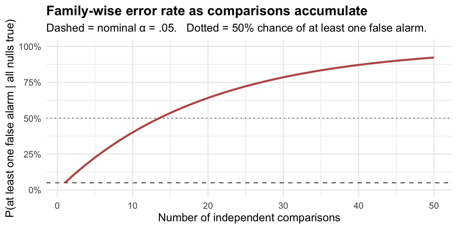
A 26% chance of finding a “significant difference” purely by chance — even when none of the differences are real. That’s the family-wise error rate (FWER), and it grows quickly with the number of comparisons:
One caveat on that 26%. The calculation assumes the six tests are independent. Pairwise comparisons among the same four groups are not independent: they share group means and, in the usual ANOVA setting, a common estimate of the error variance. So 26% is an illustration of how multiplicity accumulates, not the exact family-wise error rate for these six comparisons. (Simulating the complete null for four equal-sized groups puts the actual figure nearer 20%.) The important point is unchanged: testing many comparisons at an unadjusted \(\alpha = .05\) raises the chance of at least one false rejection, and it does so quickly.
Show the code that built this figure
tibble(n_tests =1:50) |>mutate(fwer =1- (1-0.05) ^ n_tests) |>ggplot(aes(x = n_tests, y = fwer)) +geom_line(linewidth =1.2, color ="#C05852") +geom_hline(yintercept =0.05, linetype ="dashed", color ="grey40") +geom_hline(yintercept =0.50, linetype ="dotted", color ="grey50") +scale_y_continuous(limits =c(0, 1), labels = scales::percent_format(accuracy =1)) +labs(title ="Family-wise error rate as comparisons accumulate",subtitle ="Dashed = nominal α = .05. Dotted = 50% chance of at least one false alarm.",x ="Number of independent comparisons",y ="P(at least one false alarm | all nulls true)" )
The family-wise error rate (FWER) under independent comparisons, each tested at α = .05. With just 14 comparisons, the chance of at least one false alarm exceeds 50%.
Multiple-comparison corrections exist to keep some version of the false-alarm rate under control as the number of comparisons grows.
FWER vs FDR — what each method controls
There are two fundamentally different things you might want to control:
Family-wise error rate (FWER). The probability of at least one false alarm across all comparisons. Controlling FWER at \(0.05\) means the probability of making one or more false rejections anywhere in the family is at most 5%. Note what this is not: it is not a statement about the error rate of any individual comparison. This is the conservative target — it treats a single false alarm anywhere in the family as the thing to guard against.
False discovery rate (FDR). The expected proportion of false discoveries among the hypotheses you reject. Controlling FDR at \(0.05\) means that across repeated applications of the procedure, the average false-discovery proportion is held at 5% or below. It does not guarantee that 5% or fewer of the significant findings in any one study are false — FDR is an expectation, not a per-study promise. This is the more permissive target: it accepts some false positives in exchange for catching more of the real effects.
Which to control follows from your inferential goal and from how you define the family — not simply from how many tests you happen to run. In confirmatory work, where a single false positive would be acted on directly, FWER is the appropriate target. In exploratory analyses where flagged findings will be validated by follow-up rather than acted on, FDR is often the more useful one.
The four standard methods
1. Tukey HSD — the workhorse for ANOVA
What it controls: FWER for all pairwise mean comparisons after a one-way ANOVA — exactly so when group sizes are equal (see the assumptions below).
How it works: Tukey’s Honest Significant Difference (HSD) test references the studentized range distribution, which describes the expected maximum gap between any pair of group means in a sample of \(k\) groups under \(H_0\). Comparing each observed pairwise difference to the studentized range critical value is equivalent (mathematically) to controlling the family-wise error rate at the chosen \(\alpha\) across all \(\binom{k}{2}\) comparisons.
When to use it: This is the standard choice when you want all pairwise comparisons. It is usually taught as the follow-up to a significant omnibus F, and that is a sensible workflow — but note that Tukey does not require a significant F first. TukeyHSD() controls the family of pairwise comparisons on its own, producing simultaneous intervals for every pair. For the all-pairwise case it is more powerful than Bonferroni or Holm, because the studentized range is tailored to exactly that family of comparisons. It is not, however, the most powerful FWER-controlling method available — step-down range procedures such as REGWQ can do better in some situations. Tukey is the standard recommendation because it is powerful, exact, and universally recognized, not because nothing can beat it.
Two assumptions worth stating. Tukey HSD assumes equal variances across groups, and it controls FWER exactly only when group sizes are equal. With unequal n, TukeyHSD() applies the Tukey–Kramer extension, which adjusts for the differing sample sizes; Hayter (1984) proved it is conservative, and R’s documentation describes it as giving sensible intervals for mildly unbalanced designs.
R code:
TukeyHSD(aov(y ~ group, data = my_data)) |>
  broom::tidy()
2. Bonferroni — the conservative default
What it controls: FWER, with a guaranteed (often slightly over-conservative) bound.
How it works: Test each comparison at \(\alpha / m\) instead of \(\alpha\), where \(m\) is the number of comparisons. Equivalently, multiply each p-value by \(m\) and compare to \(\alpha\).
Trade-off: Conservative — controls FWER for any set of comparisons, including non-pairwise contrasts, dependent tests, and unequal sample sizes. The cost is power: with many comparisons, the per-test threshold becomes very small and real effects get missed.
When to use it: When you have a small number of pre-planned comparisons, when the comparisons aren’t all pairwise (e.g., you’re testing a custom contrast), or when you need a method that doesn’t depend on a specific reference distribution. Easy to apply by hand; reviewers always understand it.
R code:
p.adjust(p_values, method ="bonferroni")
3. Holm-Bonferroni — improved Bonferroni
What it controls: FWER, with strong control at level ≤ α — like Bonferroni it is conservative rather than exact, but it is uniformly at least as powerful.
How it works: Order the p-values from smallest to largest. Test the smallest at \(\alpha / m\), the next at \(\alpha / (m - 1)\), the next at \(\alpha / (m - 2)\), and so on. Stop the first time a test fails to reject; declare nothing else significant. This is a step-down procedure.
Trade-off: Uniformly at least as powerful as Bonferroni — never less, often more — with the same FWER guarantee. For deciding significance, Holm dominates.
The one reason to still reach for Bonferroni: simultaneous confidence intervals. Every Bonferroni interval simply uses the same \(1 - \alpha/m\) confidence level, which is easy to compute, easy to explain, and easy for a reader to check. Simultaneous intervals corresponding to Holm-type step-down procedures do exist, but their construction is considerably less straightforward. If you are reporting adjusted intervals rather than only adjusted p-values — which this course generally prefers — plain Bonferroni is often the practical choice.
When to use it: Whenever you’d consider Bonferroni — Holm gives more power for free. The default p.adjust() choice is "holm", which is Holm-Bonferroni.
R code:
p.adjust(p_values, method ="holm") # also the p.adjust default
4. Benjamini-Hochberg (BH) — FDR control
What it controls: False discovery rate (not FWER) at the chosen level.
How it works: Order the \(m\) p-values from smallest to largest. Find the largest \(i\) such that \(p_{(i)} \leq (i / m) \cdot q\) where \(q\) is the desired FDR (e.g., \(0.05\)). Reject every null with rank \(\leq i\).
Trade-off: Substantially more powerful than FWER methods when you have many comparisons. The cost: FDR is not the same as FWER. If BH controls FDR at 5%, that means 5% of your significant findings are expected to be false alarms — not that the probability of any false alarm is 5%.
When to use it: Large-scale exploratory analyses where you expect many real effects mixed with many nulls (genomics, brain imaging, large survey data), and where the findings you flag will be followed up rather than acted on directly.
An assumption to check. BH controls FDR under independence or under a positive-dependence condition. That covers a great many realistic designs, but not all of them — under arbitrary dependence you need the more conservative Benjamini–Yekutieli procedure, available as p.adjust(p_values, method = "BY").
R code:
p.adjust(p_values, method ="BH")
Decision flowchart
Your scenario
Recommended method
All pairwise comparisons after one-way ANOVA
Tukey HSD
Pre-planned, non-pairwise contrasts; small \(m\)
Holm-Bonferroni
Many comparisons; FWER concern
Holm-Bonferroni
Many comparisons; willing to accept some false positives
Benjamini-Hochberg (FDR)
Need FWER control, no more specialised structure to exploit
Holm-Bonferroni — a strong general-purpose choice
The R function p.adjust() implements Bonferroni, Holm, BH, and several other p-value adjustments — the full list is holm, hochberg, hommel, bonferroni, BH, BY, fdr, and none. If you have computed your own comparisons and want to correct the resulting p-values, it is the one-liner.
Tukey is the exception. It is not a p-value adjustment and is not available in p.adjust(); it is a different procedure built on the studentized range. Fit the ANOVA model first, then use TukeyHSD().
Worked example
Suppose you’ve run a one-way ANOVA across four groups and computed all six pairwise t-tests. Here are the raw (uncorrected) p-values:
raw_p <-c("A vs B"=0.001,"A vs C"=0.012,"A vs D"=0.038,"B vs C"=0.142,"B vs D"=0.250,"C vs D"=0.620)tibble(comparison =names(raw_p),raw_p = raw_p,bonferroni =p.adjust(raw_p, method ="bonferroni"),holm =p.adjust(raw_p, method ="holm"),bh_fdr =p.adjust(raw_p, method ="BH")) |>mutate(across(c(raw_p, bonferroni, holm, bh_fdr), ~round(.x, 3)))
Read the table against \(\alpha = .05\) and four things stand out:
A vs B (raw \(.001\)) survives every correction, landing at \(.006\) under all three. A p-value that small has enough margin to absorb a sixfold penalty.
A vs C (raw \(.012\)) survives only under BH (\(.036\)). Both FWER methods reject it — Bonferroni at \(.072\), Holm at \(.060\). Holm’s advantage over Bonferroni is visible here, but it is not large enough to carry this comparison across the threshold.
A vs D (raw \(.038\)) survives nothing, BH included (\(.076\)). A raw p-value just under \(.05\) has almost no margin once six comparisons are accounted for. Being significant before correction says very little.
The remaining three stay non-significant throughout. No method ever creates significance — corrections only ever move p-values up.
Where the FWER-vs-FDR choice actually bites here: A vs C. It is significant under BH (\(.036\)) and not under Holm (\(.060\)), and that single disagreement is the whole trade-off in miniature. If a false alarm would be costly — a clinical recommendation, a confirmatory claim — Holm is the right call, and you report A vs B alone. If this is exploratory work where the reward is generating leads and you accept that roughly 5% of what you flag will be false, BH lets you carry A vs C forward as worth a closer look.
Notice also how little the two families disagree at this scale: with six comparisons, BH and the FWER methods reach the same verdict on five of them. BH is perfectly legitimate with six hypotheses — its power advantage over FWER methods is simply far more consequential when the family runs to hundreds or thousands.
References
Benjamini, Y., & Hochberg, Y. (1995). Controlling the false discovery rate: A practical and powerful approach to multiple testing. Journal of the Royal Statistical Society Series B, 57(1), 289–300.
Hayter, A. J. (1984). A proof of the conjecture that the Tukey–Kramer multiple comparisons procedure is conservative. The Annals of Statistics, 12(1), 61–75.
Holm, S. (1979). A simple sequentially rejective multiple test procedure. Scandinavian Journal of Statistics, 6, 65–70.
Tukey, J. W. (1953). The problem of multiple comparisons. Unpublished manuscript, reprinted in Tukey, J. W. (1994), The Collected Works of John W. Tukey, Vol. VIII (pp. 1–300). Chapman & Hall.