| variable_name | label | notes |
|---|---|---|
| id | inmate ID | NA |
| years | sentence length in years | NA |
| black | race (1 = black, 0 = white) | NA |
| afro | rating for afrocentric features | inmate photo rated by ~35 CU undergraduate students; raters assigned a single, global assessment of the degree to which each face had features that are typical of African Americans, using a scale from 1 (not at all) to 9 (very much) |
| primlev | seriousness of primary offense | based on Florida’s rating system, higher numbers indicate more serious felonies |
| seclev | seriousness of secondary offense | based on Florida’s rating system, higher numbers indicate more serious felonies |
| nsecond | number of secondary offenses | NA |
| anysec | indicator for any secondary offenses (1 = yes, 0 = no) | NA |
| priorlev | seriousness of prior offenses | based on Florida’s rating system, higher numbers indicate more serious felonies |
| nprior | number of prior offenses | NA |
| anyprior | indicator for any prior offenses (1 = yes, 0 = no) | NA |
| attract | rating for attractiveness | inmate photo rated by ~35 CU undergraduate students |
| babyface | rating for babyface features | inmate photo rated by ~35 CU undergraduate students |
Apply and Practice Activity
Blair Replication Explore Polynomials
Introduction

Building on our replication of the Blair et al. study — this Apply and Practice Activity will delve into the curvilinear relationship between the seriousness of the primary crime committed by inmates and the sentence length given by the judge. Blair and colleagues hypothesized that sentence length should exhibit a non-linear, ramping up pattern, as the seriousness of the offense increases. As such, they asserted that at low levels of seriousness, each one unit increase in seriousness of the crime should have a small increasing effect on sentence length. However, at higher levels of seriousness, each one unit increase in seriousness of the crime should have a larger increasing effect on sentence length.
To address this unique relationship, we will explore the implementation of polynomial regression models — a powerful method capable of capturing such non-linear effects. Through this activity, you will gain hands-on experience in fitting a polynomial model, evaluating its efficacy in tackling this complex relationship, and, most importantly, mastering the skill of interpreting the effects generated by the fitted model.
As a reminder, here is a list of the variables in the data frame:
Please follow the steps below to complete this activity.
Step by step directions
Step 1
Open up the blair_replication project in the Posit Cloud.
Step 2
In the Files tab of the lower right quadrant of RStudio, open up the blair_replication_setup.qmd document that you created earlier. Save a copy of this — call it blair_replication_poly.qmd (click File -> Save As…, then provide the new name). In the YAML header, change the title to: “Blair Replication: Explore Polynomials”. We’ll do all of the work for this activity in this new version — blair_replication_poly.qmd.
Step 3
Click the down arrow beside Run in the top menu of the RStudio session, and then choose Restart R and Run All Chunks.
Step 4
Use the output from the code chunk under the header # Describe variables (which uses the skim() function to provide descriptive statistics for the variables).
Match the variables up with the description of variables in the Introduction. Write a few of sentences to describe the descriptive statistics — focus on the variables sentence length in years (years) and seriousness of the primary crime (primlev). Describe what the variables represent and describe the descriptive statistics in sentence form. Put these sentences in the white space of your analysis notebook underneath the skim() output.
Step 5
In the Blair and colleagues study, they included quadratic polynomial terms (i.e., \(x_i\) and \(x_i^2\)) for each of the seriousness measures — that is, for the primary crime (primlev), the secondary crime(s) (seclev), and for prior crimes (priorlev). In this Apply and Practice Activity, we will fit the quadratic relationship between seriousness of the primary crime (primlev) and log sentence length (lnyears).
As you learned in Module 15, when including a quadratic term for a predictor of interest, one creates a new version of the predictor that is the square of itself — for example primlev2 = primlev^2, then both the initial version of the predictor and this squared version of the predictor are included in the regression model as predictors. This allows for a curvilinear effect of the variable of interest on the outcome. By allowing the effect of seriousness of the offense to have a quadratic effect, Blair and colleagues allowed for their assertion that:
the length of the sentence ought to increase dramatically as the seriousness of the offense increases.
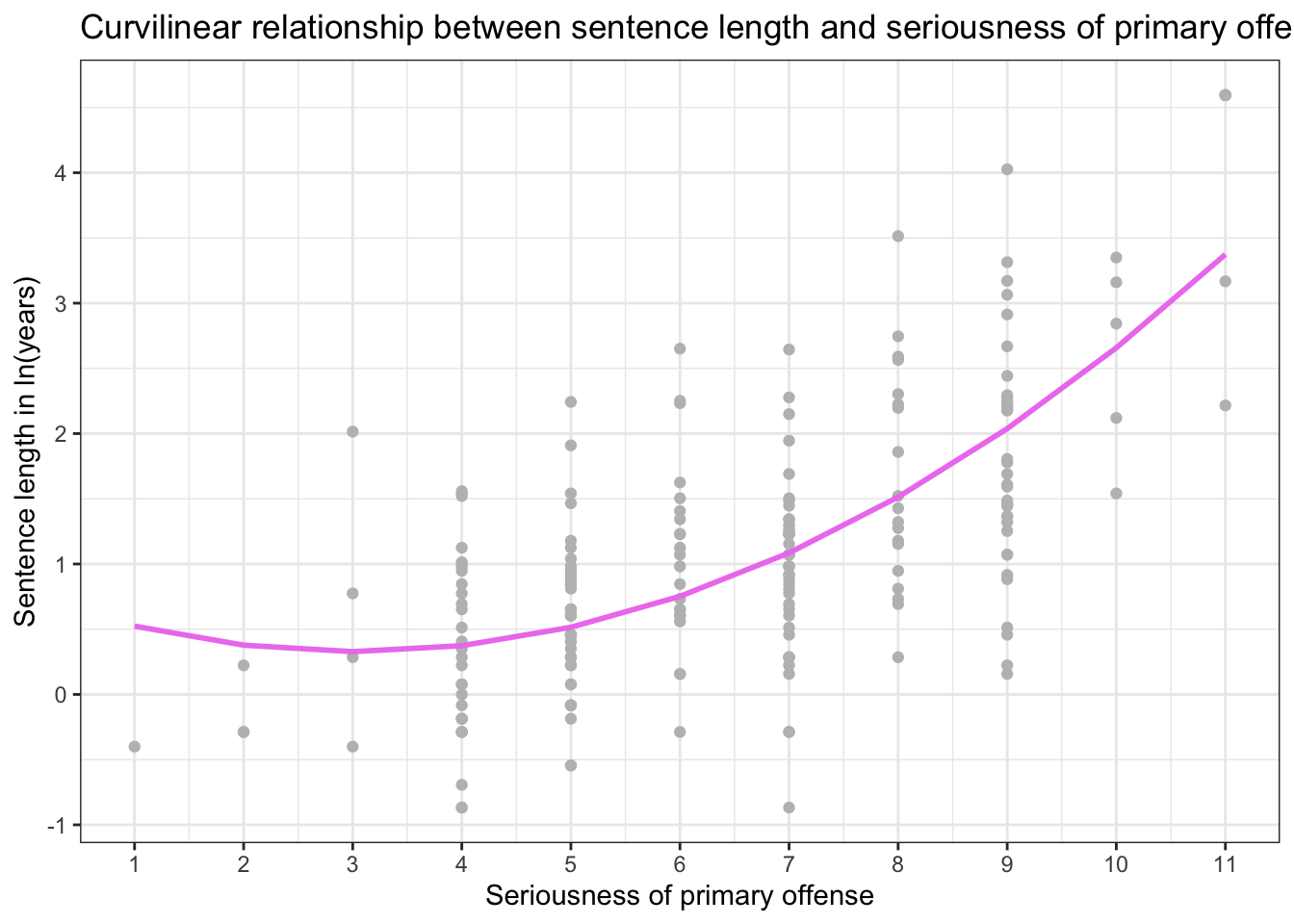
That is, that seriousness should not be linearly related to sentence length, but rather non-linearly related such that as seriousness increased, sentence length ramped upward. You can see this effect in the example graph below. At higher levels of seriousness (e.g., above about a score of 5) each one unit increase in seriousness is associated with a larger increase in log sentence length than at lower levels of seriousness.
For example, take a look at the slope of the violet line between a seriousness score of 3 and 4 on the x-axis — here the slope is relatively flat. Now, look at the slope of the violet line between a seriousness score of 8 and 9. Here, the slope of the line is quite steep. This indicates that the change in log sentence length for a one-unit increase in seriousness is different at low levels of seriousness as compared to high levels of seriousness.

Below the last code chunk, create a first level header called
# Examine the curvilinear effect of primlev on lnyears
Then, a second level header called
## Prepare lnyears and the polynomial term
Then insert a code chunk.
Inside the code chunk form two new variables:
lnyears — which is the log of years
primlev2 — which is primlev squared (i.e.,
primlev2 = primlev*primlevorprimlev2 = primlev^2)
Step 6
Now, we can fit the polynomial regression model to examine the quadratic effect of seriousness of crime on sentence length.
Create a second level header called
## Fit the polynomial regression model
Then insert a code chunk.
Inside the code chunk, fit a lm() model (name the model poly). Regress lnyears on primlev and primlev2. Use tidy() to obtain the model output.
Step 7
Interpretation of a polynomial regression model takes care. In this section you will work through interpreting the model. Recall the basic structure of a quadratic regression model:
\[ \hat{y_i} = {b_0} + ({b_1}\times{x_i}) + ({b_2}\times{x^2_i}) \]
Where \({x_i}\) refers to primlev and \({x^2_i}\) refers to primlev2.
The graph of a quadratic regression model is the shape of a parabola. This shape can be mound shaped (i.e., an inverted U) or bowl shaped (i.e., a U). The sign of the squared term (i.e., \({b_2}\) in the equation or the estimate for primlev2) indicates whether the shape is a mound or bowl. If \({b_2}\) is positive then the parabola is bowl shaped and if \({b_2}\) is negative then the parabola is mound shaped.
Is the parabola for our example mound or bowl shaped? In your analysis notebook, underneath the model results of poly, write a sentence or two to describe the shape of the parabola given the model estimates.
Step 8
The estimate for the intercept is the predicted log sentence length for an inmate who committed a primary offense rated as 0. Please note that the lowest primary severity score in the sample is 1 — and when we actually fit the Blair models in a later Apply and Practice Activity we will center the primlev variable — but for now, we will leave it as is in order to keep things simple.
Interpreting the intercept, we see that the predicted natural log of sentence length in years when the seriousness of the primary offense is 0 is 0.765 ln(years).
This predicted score is in log sentence length in years — but recall from our earlier Apply and Practice Activity on logarithms that we can take the antilog to convert back to the origical metric — i.e., years.
In the code chunk underneath the specification of the poly model, compute the predicted sentence length in years when the seriousness of the primary offense is 0. Then write a sentence to describe what the value represents.
Step 9
There is a value of \(x_i\) along the curve when the slope drawn tangent to the line is 0. In other words, this is the point at which the predicted value of \(y_i\) (i.e., fitted value or y-hat) takes a maximum value if the parabola is a mound or a minimum value if the parabola is a bowl. This point is called the vertex, and the x-axis coordinate for the vertex can be estimated with the following formula:
\[ {-b_1} \div (2\times{b_2}) \]
Use the results of the polynomial regression model to calculate the x-coordinate of the vertex. Show your method of calculating this value. Then, write a sentence or two in your analysis notebook to describe what this value represents.
Step 10
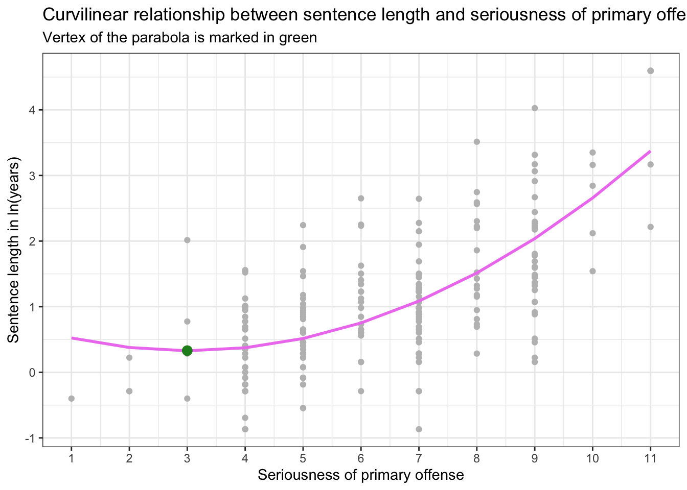
The vertex is marked on the graph below in green — it is the score for primlev when lnyears is at it’s minimum.

Step 11
The slope of a line drawn tangent to the parabola at a certain \(x_i\) score is estimated by:
\[ {b_1} + (2\times{b_2}\times{x_i}) \]
We can calculate the slope drawn tangent to the line at any desired \(x_i\) score (i.e., score for primlev).
For example:
When primlev = 3 the slope is: \(-.289 + (2\times.048\times3) = 0.00\)
Your turn: Calculate the slope drawn tangent to the parabola when primlev = 6.5 and when primlev = 10. Show your work to calculate these scores and then write a sentence or two in your analysis notebook to describe what these values represent.
Step 12
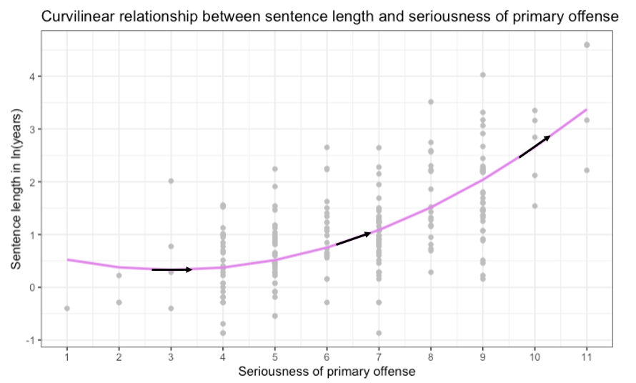
Comparing the three calculated slopes (when primlev = 3, 6.5, and 10), we can see that as the seriousness of offense increases, there is a ramping up of the effect of seriousness on log sentence length in years. These three slopes are overlaid as black arrows on the graph below.

Step 13
Recall from our lesson on interpretation of models with an outcome that has been transformed by taking the natural log, that we can interpret a slope in terms of the unit change in the outcome in the transformed metric (i.e., ln(years)), but we must interpret the slope in terms of percent change in the raw metric (i.e, percent change in years).
For example, let’s take the slope that we just calculated when primlev is 6.5 — which is 0.33. I’ll input that as the slope in the code that calls the function below.
# function --- don't change anything here
ln.y <- function(slope, x_chg) {
  new_slope <- 100 * (exp(slope * x_chg) - 1)
  return(new_slope)
}

# input your slope from the regression output, and the desired change in x
ln.y(slope = 0.33, x_chg = 1)
[1] 39.09681This value, indicates that we expect the sentence length in years to be about 39% larger as we move from a score of 6.5 to 7.5 on primlev.
For very serious crimes (primlev = 10), what is the expected change in sentence length in years as we move from a score of 10 to 11?
In your analysis notebook, add a second level header called
## Compute predicted score
Copy and paste the code chunk above into your analysis notebook — then use the ln.y() function to answer the question. Write a sentence or two to describe the answer.
Step 14
To further grow our intuition about polynomial models, let’s calculate the predicted sentence length in years for prototypical levels of primlev.
In your analysis notebook, add a second level header called
## Graph the fitted model
Then insert a code chunk. Copy and paste the code below. Run the code chunk and study the predicted scores in both lnyears and years for each level of primlev. Underneath the table, write a few sentences to describe what’s happening in the code. Also describe the results.
# Create a data frame of desired scores for primlev
primlev_scores <-
  tibble(primlev = seq(from = 1, to = 11, by = 1))

# Compute squared version
primlev_scores <-
  primlev_scores |>
  mutate(primlev2 = primlev^2)

# Use predict function
pred_lnyears <- predict(poly, newdata = primlev_scores)

# Join together the primlev prototypical values and predicted lnyears (tibble creates a data frame from the two vectors)
pred_df <- tibble(primlev_scores, pred_lnyears)

# Exponentiate the predicted values
pred_df <-
  pred_df |>
  mutate(pred_years = exp(pred_lnyears))

pred_df
Now, add another code chunk. In this code chunk create a graph using the pred_df data frame of predicted scores that we just created. In this graph map primlev to the x-axis and pred_years to the y-axis. Request both geom_point() and geom_line() geometries. Give the graph the following title: “Fitted relationship between seriousness of primary offense and sentence length in years”.
In your notebook, take a few minutes to describe the effect of seriousness of the primary offense on sentence length. Use what you’ve learned in this lesson about quadratic models to describe the relationship in your own words.
Step 15
Now that you’ve completed all tasks, to help ensure reproducibility, click the down arrow beside the Run button toward the top of your screen then click Restart R and Clear Output. Scroll through your notebook and see that all of the output is now gone. Now, click the down arrow beside the Run button again, then click Restart R and Run All Chunks. Scroll through the file and make sure that everything ran as you would expect. You will find a red bar on the side of a code chunk if an error has occurred. Taking this step ensures that all code chunks are running from top to bottom, in the intended sequence, and producing output that will be reproduced the next time you work on this project.
Now that all code chunks are working as you’d like, click Render. This will create an .html output of your report. Scroll through to make sure everything is correct. The .html output file will be saved along side the corresponding .qmd notebook file.