Data Wrangling

Module 4

Learning Objectives

By the end of this module, you should be able to:

• Explain what data wrangling is and why it is important for data analysis
  
• Understand how functions from the dplyr package support modular, readable workflows
  
• Chain together functions using the pipe operator (|>) to express multi-step wrangling operations
  
• Write clear and efficient pipelines that combine multiple tidyverse functions to clean and explore data
  
• Recognize how dplyr verbs preserve a “data in, data out” logic that supports reproducibility
  
• Apply wrangling techniques to filter, transform, and summarize real datasets in preparation for analysis or visualization

Overview

To wrangle data is to clean and prepare data for analysis. Our goal is to get the data into a tidy shape that can be readily plotted and analyzed. I like to think about data analysis in terms of painting a room. In painting, an excellent result comes from careful and thorough preparation. About 90% of painting is preparation — cleaning the walls, taping off trim, protecting the floor, getting the right tools, etc. Data analysis is similar — and data wrangling is the preparation.

Neglecting this step or performing it haphazardly can greatly compromise the quality of your data analysis results. Thus, recognizing the significance of data wrangling and investing ample effort in this stage will set the foundation for robust and meaningful data analysis.

In this Module, you’ll learn to use functions from the dplyr package to build a modular, readable workflow — one where each function performs a specific task, and steps are linked together to form a clear sequence of transformations. This approach helps you write code that is easier to understand, troubleshoot, and adapt as your analysis evolves. These workflows follow a “data in, data out” logic: each function takes a data frame as input, applies a transformation, and returns a data frame as output. This structure not only makes your code easier to understand and maintain, but also reflects the natural, step-by-step way we approach real-world data analysis.

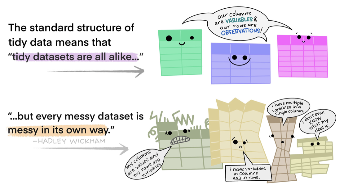
Tidy Data

Tidy data is a concept introduced by statisticians Hadley Wickham and Garrett Grolemund, they outline a standard and consistent way of organizing and structuring data for analysis. The tidy data approach promotes a specific data format that facilitates efficient data manipulation, visualization, and modeling. The principles of tidy data are often associated with the tidyverse ecosystem of R packages, including dplyr and tidyr.

Artwork by @allison_horst

Tidy data principles

According to the principles of tidy data, a data frame is considered tidy if it satisfies the following criteria:

Tidy Principle 1 — Each variable has its own column: Each variable or attribute is represented by a separate column in the data frame. This means that different types of information should be organized into distinct columns. For example, here’s an untidy data frame where address is a string recorded in a single column.

And, here is the data frame in a tidy form. In the tidy data frame, street, city, state and zipcode are in separate columns. This makes working with these data much easier — for example, this structure facilitates choosing certain States or merging in other information that pertains to participants’ zip codes.

Tidy Principle 2 — Each observation has its own row: Each individual observation or data point is represented by a separate row in the data frame. This ensures that each row contains all relevant information for a specific observation. For example, in the untidy data frame below each row represents a participant, and the anxiety levels before and after the intervention are stored in separate columns. This violates the tidy data principle, as each observation should have its own row.

To transform the untidy data into tidy data, we create a new data frame where each row represents a single observation. In this case, each observation is a participant’s anxiety level at a specific time point. In the tidy data example, we have three columns: participant, time, and anxiety. Each row represents a specific observation of anxiety level, with the participant column indicating the participant’s ID, the time column indicating the time point (“pre” or “post”), and the anxiety column containing the corresponding anxiety level at that time point. This way, each participant’s anxiety levels at each time point have their own row in the tidy data, and all the relevant information for each observation is contained within that row. Later, you’ll see examples of how this structure better facilitates graphing and modeling.

Tidy Principle 3 — Each cell holds a single value: Each cell in the data frame contains a single value. There should be no cells that contain multiple values or combinations of values. For example, consider this untidy data frame where a weight column contains weight measurements recorded in both kilograms and pounds.

To transform the untidy data into tidy data, we create a new column (i.e., variable), weight_kg, which converts all weight measurements to a consistent unit (kilograms).

Artwork by @allison_horst

By organizing data in a tidy format, it becomes easier to perform various data manipulation tasks. Tidy data simplifies tasks such as filtering, sorting, grouping, and aggregating data. It also facilitates seamless integration with the tidyverse tools, making it straightforward to apply functions like dplyr’s filter(), mutate(), and summarize() — all of which we’ll learn about in this Module.

Getting data into a tidy shape should be the first priority when working with a new data frame. While it’s common to encounter untidy data frames that require substantial tidying efforts, it’s important to recognize that adhering to the principles of tidy data is invaluable and will save you time in the long run. The benefits of getting your data into a tidy shape up front far outweigh the time investment needed. Adhering to the principles of tidy data promotes code readability, reproducibility, and enables effective collaboration among data analysts and scientists. It helps eliminate ambiguity, reduces errors, and streamlines the data wrangling process, ultimately leading to more efficient and reliable data analysis. Hooray!!

Introduction to the Data

The opioid epidemic

The opioid epidemic in America signifies a profound and alarming surge in the misuse, addiction, and fatal overdoses associated with opioids. This includes the misuse of prescription opioids as well as the proliferation of illicit substances such as heroin and potent synthetic opioids like fentanyl. The opioid epidemic has swiftly evolved into a severe public health crisis, leaving devastating consequences in its wake throughout the United States. The scale and impact of this crisis have captured widespread attention and urgency, necessitating comprehensive efforts to address its multifaceted challenges.

The roots of the opioid epidemic can be traced back to the late 1990s when there was a surge in the prescription of opioid pain relievers. Pharmaceutical companies reassured the medical community that these medications were safe and had low risks of addiction. Consequently, there was widespread overprescribing and a subsequent increase in opioid availability.

Prescription opioids are medications primarily used to manage severe pain. Examples include oxycodone, hydrocodone, morphine, and fentanyl. Many individuals who initially received these medications for legitimate medical reasons became addicted, leading to increased dependence and misuse.

As prescription opioids became harder to obtain or more expensive, some individuals turned to heroin as a cheaper and more accessible alternative. Additionally, illicitly manufactured synthetic opioids, particularly fentanyl, have been increasingly involved in overdose deaths. Fentanyl is significantly more potent than other opioids (it is estimated to be 50 to 100 times more potent than heroin or morphine).

The graph below shows the three phases of the opioid epidemic.

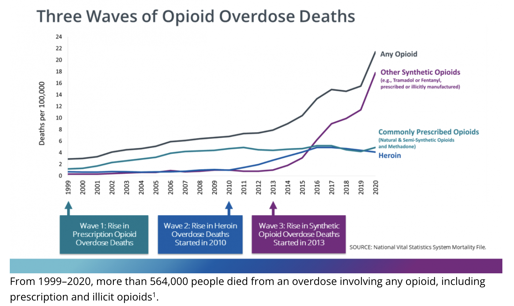
The opioid epidemic has resulted in a staggering number of overdose deaths. According to the Centers for Disease Control and Prevention (CDC), between 1999 and 2022, approximately 727,000 individuals lost their lives due to opioid overdoses. The crisis has further intensified in recent years, with an alarming rise in overdose deaths attributed to synthetic opioids, including fentanyl.

The opioid epidemic has had far-reaching consequences for individuals, families, and communities. It has led to an increase in infectious diseases like HIV and hepatitis C, strains on healthcare and criminal justice systems, and a significant economic burden due to lost productivity and increased healthcare costs.

To provide additional context, please watch the following video from Last Week Tonight with John Oliver. Please note that the video contains some lewd language, you can skip the video without it affecting your ability to understand the material in this Module. If interested, you can also peruse this National Public Radio article and this Nature paper that also provide context.

ARCOS data

In July of 2019, The Washington Post revealed that roughly 76 billion oxycodone and hydrocodone pills were bought and sold in the United States between 2006 and 2012. This valuable data was sourced from the Automation of Reports and Consolidated Orders System (ARCOS), a comprehensive database maintained by the U.S. Drug Enforcement Administration (DEA) that meticulously tracks the distribution of every pain pill sold within the country. The ARCOS data had been strictly confidential until The Washington Post (WAPO) publication, with the DEA receiving the information directly from registrants. However, after a protracted legal battle, the Sixth Circuit Court of Appeals ordered the release of the data, enabling the WAPO to access and publish it. This unprecedented release shed light on a previously undisclosed aspect of the opioid crisis, providing valuable insights into the distribution and consumption patterns of opioids.

In this Module we’re going to work with the WAPO compiled data repository. We will use the county level data. Each county in the US has up to nine rows of data in this data frame, one for each year from 2006 to 2014. The table below describes the variables that we will utilize:

Variable	Description
fips	A 5 digit code that identifies each county
county	County name
state	State abbreviation
year	Corresponding year for data
number_pills	The number of Oxycodone & Hydrocodone pills purchased by pharmacies in the county
population	The total number of people living in the county

Let’s load the libraries that we will need in this Module.

library(skimr)
library(here)
library(tidyverse)

Now, we can import the data frame, which is called opioid_counties.Rds.

opioid_counties <- read_rds(here("data", "opioid_counties.Rds")) 

Let’s take a glimpse at the data to see the variable types (e.g., character, integer).

opioid_counties |> 
  glimpse()

Rows: 27,758
Columns: 6
$ fips         <chr> "45001", "45001", "45001", "45001", "45001", "45001", "45…
$ county       <chr> "ABBEVILLE", "ABBEVILLE", "ABBEVILLE", "ABBEVILLE", "ABBE…
$ state        <chr> "SC", "SC", "SC", "SC", "SC", "SC", "SC", "SC", "SC", "LA…
$ year         <int> 2006, 2007, 2008, 2009, 2010, 2011, 2012, 2013, 2014, 200…
$ number_pills <int> 363620, 402940, 424590, 467230, 539280, 566560, 589010, 5…
$ population   <int> 25821, 25745, 25699, 25347, 25643, 25515, 25387, 25233, 2…

Here, we see that three of the variables are character variables — fips, county, and state. The remaining three — year, number_pills, and population — are integers.

This data frame is very large, and printing it out takes a lot of resources. However, we can peek at the first rows with the head() function. The head() function, by default, will display the first 6 rows of data. However, we can add the n argument to the function to change that number. For example, n = 18 requests 18 rows be printed. Note that the function tail() works in the same way, but shows the last rows in the data frame.

Tip

Every R function ends with parentheses — for example, head(). Inside the parentheses, we provide arguments, which are instructions that tell the function what to do. For instance, `head(n = 18)` tells R to return the first 18 rows of the dataset.

To learn what arguments are available for a function, you can type ?head or help(head) into the console to view the documentation (it will show up in the Help tab of the lower right quadrant of RStudio).

In RStudio, placing your cursor inside the parentheses and pressing Tab can also be a helpful way to explore arguments — especially for functions from the tidyverse and other packages. For example, type aes() — then with the cursor inside the parentheses press Tab. It will give you a list of arguments that are allowed for this function — which, recalling from Module 02, is a function that can be used in ggplot2 to map variables to elements of the plot.

opioid_counties |> 
  head(n = 18)

The dplyr Functions to Wrangle Data

dplyr is a R package that is part of the tidyverse — it’s the workhorse for wrangling data. Overall, dplyr plays a crucial role in data wrangling by providing a concise and consistent set of functions for data manipulation and transformation in R. It simplifies complex data wrangling tasks, improves code readability, and enhances productivity.

In this Module, we will explore the following dplyr data wrangling functions:

• Choose certain cases (rows) in your data frame with filter()
• Choose certain variables (columns) in your data frame with select()
• Collapse many values down to summaries with group_by() and summarize()
• Handle missing data with drop_na()
• Create or modify variables with mutate()
• Give variables a new name with rename()
• Order your cases (rows) with arrange()
• Pivot data from wide to long with pivot_longer() and from long to wide with pivot_wider()
• Merge two data frames together with left_join()
• Create a new variable based on conditions of existing variable(s) using case_when()

The filter() function

Artwork by @allison_horst

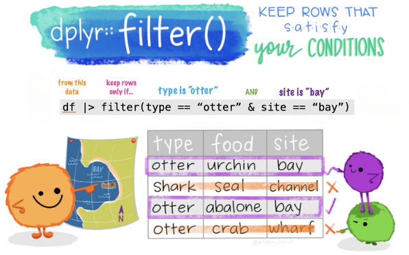
The filter() function is used to choose specific rows of data that meet certain conditions. R provides a standard set of selection operators:

• > is “greater than”

• >= is “greater than or equal to”

• < is “less than”

• <= is “less than or equal to”

• != is “not equal to”

• == is “equal to”

Boolean operators¹ are also permitted:

• & is “and”

• | is “or”

• ! is “not”

A single filter

First, let’s use filter() to create a new data frame called opioid_counties2014, that starts with the opioid_counties data frame that we just read in, then filters the data to include only rows where the year is 2014.

opioid_counties2014 <- 
  opioid_counties |> 
  filter(year == 2014)

opioid_counties2014 |> 
  head()

Notice the use of the double equals sign (==). In R, this is the comparison operator — it checks whether the value of year is equal to 2014. This is different from the single equals sign (=), which is used to assign values (like in function arguments or when creating a new variable). So:

• year == 2014 asks: “Is the year equal to 2014?” (comparison)

• year = 2014 would try to assign 2014 to year, which is not what we want when filtering rows.

• So, when using filter() to keep only rows that meet a condition, we use == to test for equality.

Note also that by assigning a new data frame name (opioid_counties2014), we create a new data frame that contains the filtered results. If instead, you simply wanted to overwrite the existing data frame with your filter selections, then you’d instead write:

opioid_counties <- 
  opioid_counties |> 
  filter(year == 2014)

Moving on, let’s consider some other options that might be of interest. You can replace filter(year == 2014) in the code above with the following code to accomplish different results:

• filter(year == 2013 | year == 2014) to create a data frame where year equals 2013 or 2014

• filter(year != 2006) to create a data frame that excludes year 2006 but keeps the others

• filter(year < 2010) to create a data frame that keeps all years less than 2010

• filter(year >= 2010 & year <= 2013) to create a data frame of years 2010, 2011, 2012, and 2013

• filter(year %in% c(2010, 2012, 2014)) to create a data frame of years 2010, 2012, and 2014

A few notes about these options: In the following code, filter(year %in% c(2010, 2012, 2014)), the %in% operator checks whether the values in the year column are present in the vector² c(2010, 2012, 2014). It’s like asking the question, “Does the year match any of these specific values: 2010, 2012, or 2014?, If the answer is TRUE — keep the row, if the answer is FALSE — remove the row.

Multiple filters

We can filter the data frame on more than one variable. Next, let’s create a new data frame called opioid_counties2014_CO, that includes:

1. only counties in Colorado (CO), and
2. only rows where year is equal to 2014.

opioid_counties2014_CO <- 
  opioid_counties |> 
  filter(state == "CO" & year == 2014)

opioid_counties2014_CO |> 
  head()

What if instead we wanted years 2010 to 2014? We could accomplish this by swapping the filter() call above with the following:

filter(state == "CO" & (year >= 2010 & year <= 2014))

Let’s break this down:

• state == "CO" keeps only rows where the state is Colorado. Note that when referring to a character variable, like state, you must put the value of interest in quotation marks.

• year >= 2010 & year <= 2014 keeps only rows where the year is between 2010 and 2014, inclusive. The parentheses help group the year conditions together, so R knows to evaluate them as one combined test.

• The & in the middle says: keep only rows where both conditions are true — the state is Colorado and the year is in the right range.

• Think of it like saying: “Give me the rows where the state is Colorado and the year is somewhere between 2010 and 2014.”

Using these techniques, you can filter your data frame on as many conditions as you need.

Warning

Always take a look at the resulting data frame to make sure your code performed the right task! Don’t just trust that the code worked — save yourself headaches — and verify!

The select() function

Artwork by @allison_horst

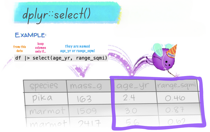
The select() function is used to select/choose only certain columns (i.e., variables) in your data frame. Let’s choose the columns/variables state, county, and number_pills — we’ll save the subsetted data frame as opioid_counties_subset.

opioid_counties_subset <- 
  opioid_counties |> 
  select(state, county, number_pills)

opioid_counties_subset |> 
  head()

You can also use select() to reorder variables. For example, if you simply wanted to move state, county, and number_pills to the front of your data frame, but still keep the other variables, you could modify the select() function above as follows:

select(state, county, number_pills, everything())

The everything() function puts all the other variables after the three specifically mentioned. This can be helpful if you want to be able to readily see the subset of variables you will be working with — but don’t want to remove the others.

There are other tidyselect helper functions that can be quite useful in certain situations, these include:

• starts_with(): Starts with a certain prefix.

• ends_with(): Ends with a certain suffix.

• contains(): Contains a literal string.

• num_range(): Matches a number range.

We’ll see a demonstration of this later in the Module. But here’s a quick example:

Imagine you have a data frame with longitudinal data, where each person has a set of variables measured at three time points.

• The time 1 variables begin with “T1”,

• the time 2 variables with “T2”, and

• the time 3 variables with “T3”.

If you wanted to select only the time 1 variables, you could use:

select(starts_with("T1"))

As another example, imagine you had a series of variables that started with “neuro” and ended with a number — e.g., neuro1, neuro2, neuro3, neuro4, neuro5. If you wanted to select neuro2, neuro3, and neuro4 — you could include:

select(num_range("neuro", 2:4))

The summarize() function

Artwork by @allison_horst

The summarize() function is used to summarize data — for example, to create summary statistics like a mean, a sum, or a standard deviation.

Compute summary statistics

Let’s compute the total number of opioid pills recorded across all counties and years. In the code below, I use na.rm = TRUE to indicate that I want R to remove cases (i.e., rows of data) with missing data on the variable being summarized and compute the specified statistic on the remainder of cases. This is necessary if there is missing data on the variable you are summarizing.

Note that in these examples, I don’t assign a name to the output, I’m simply reading in the data frame and asking it to be summarized — R will print out the requested results but the original data frame will remain unchanged.

opioid_counties |> 
  summarize(sum_number_pills = sum(number_pills, na.rm = TRUE))

The pharmaceutical companies blanketed the US with over 98 billion (98,244,239,934) opioid pills between 2006 and 2014! There were about 310 million people in the US during these years — so that’s over 300 pills per person!

Use drop_na() to remove missing cases before summarizing

Rather than using the argument na.rm = TRUE, we could use drop_na() to remove cases (i.e., rows) with missing data prior to summarizing. This will produce the same result as earlier, but demonstrates an alternative approach to handling missng data. Here’s an example of this approach:

opioid_counties |> 
  drop_na(number_pills) |> 
  summarize(sum_number_pills = sum(number_pills))

group_by() & summarize()

Artwork by @allison_horst

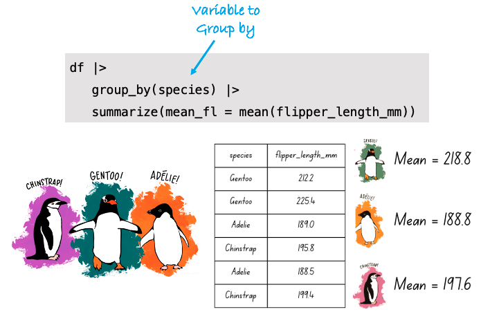
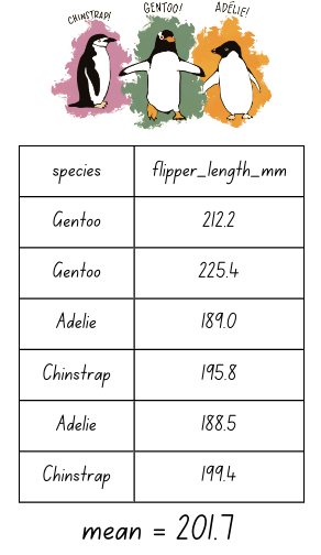
The group_by() function is used to group your data by a salient variable. Once grouped, functions can be performed by group. Let’s compute summary statistics by a grouping variable — specifically, we’ll group by year and then compute the mean and median for number of pills for each year.

opioid_counties |> 
  group_by(year) |> 
  summarize(mean_number_pills = mean(number_pills, na.rm = TRUE),
            median_number_pills = median(number_pills, na.rm = TRUE)) 

In 2006, the average number of pills recorded per county was 2,645,410, while the median was much lower at 744,830. What might this large gap between the mean and median suggest about the shape of the distribution?

We can save the object produced by our code. For example, let’s create a new data frame, called sum_pills_year that calculates the total number of pills sold each year and stores the sum as a variable in the data frame called total_pills. The result is a data frame with one row of data for each observed year, along with the total number of pills sold in that year across all counties.

sum_pills_year <- 
  opioid_counties |> 
  group_by(year) |> 
  summarize(total_pills = sum(number_pills, na.rm = TRUE))

sum_pills_year

This is a very useful function of summarize(). For example, once the summary statistics by year are produced, the resultant data frame (i.e., sum_pills_year) can be used to create a line graph to visualize the change in pills purchased across time.

Create a line graph of the result

sum_pills_year |> 
  ggplot(mapping = aes(x = year, y = total_pills)) +
  geom_line(color = "#34495E") +
  theme_bw() +
  labs(title = "Change in total number of opioid pills purchased from 2006 to 2014?",
       y = "Number of opioid pills puchased",
       x = "Year")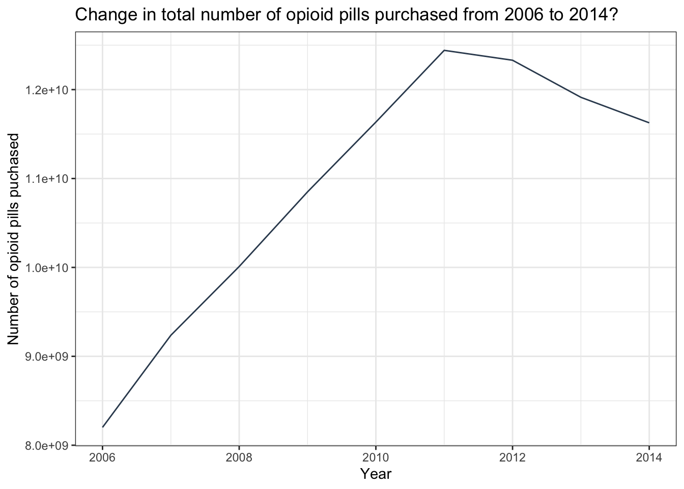 

This graph shows a precipitous increase in pills being purchased by U.S. pharmacies from 2006 to 2011, and then a slight falling back through 2014. Unfortunately, just as public health officials started realizing there was a major problem, a different opioid (heroin), stepped in to fuel the epidemic. To learn more, take a look at this CDC report.

The mutate() function

Artwork by @allison_horst

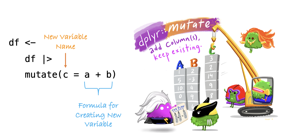
The mutate() function is used to create new variables. This is a highly versatile function that you will use over and over again.

Create a new variable that is a transformation of another

Let’s add a new variable to our data frame called pills_per_capita, which will represent the number of opioid pills per person within each county. “Per capita” is a Latin term that translates to “per person.” It is commonly used in statistics, economics, and various social sciences to provide a measurement or comparison that accounts for the number of individuals in a population. This term allows for a more meaningful comparison of data across different populations or groups, by normalizing data based on population size.

In this example, our calculation will be performed for each row, enabling a per capita comparison across the counties. By using the same name for the data frame in our assignment, we ensure that this new variable is seamlessly integrated into the existing structure, enhancing our data frame without creating a separate data frame.

opioid_counties <- 
  opioid_counties |> 
  mutate(pills_per_capita = number_pills/population) 

opioid_counties |> 
  head()

Let’s further modify our new variable pills_per_capita by rounding to the nearest tenth. We can use the round() function to accomplish this, which rounds a number to a specified number of decimal places. The round() function takes two arguments: the variable you want to round, and the number of decimal places to which you want to round. To round to the nearest tenth, you would set the number of decimal places to 1 (digits = 1). To round to the nearest hundredth, set the number of decimal places to 2 (digits = 2).

Here’s the revised code with this addition:

opioid_counties <- 
  opioid_counties |> 
   mutate(pills_per_capita = round(number_pills / population, digits = 1))

opioid_counties |> 
  head()

The rename() function

Artwork by @allison_horst

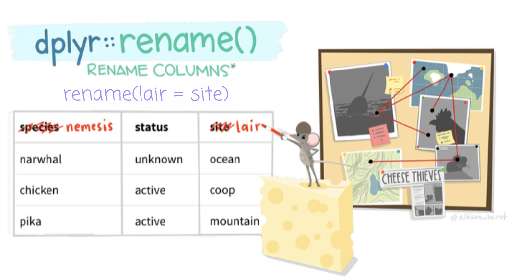
The rename() function is used to rename variables in a data frame. For example, let’s say we want to rename number_pills to opioid_pills. The syntax for rename() places the new name on the left and the existing (old) name on the right, like this: rename(new_name = old_name).

So in our case, we would write:

opioid_counties_rename <- 
  opioid_counties |> 
  rename(opioid_pills = number_pills)

opioid_counties_rename |> 
  head()

This replaces the old variable name number_pills with the new name opioid_pills in the new data frame.

Notice here that I created a new data frame, so the original data frame will be unchanged. Instead, if you wanted to change the name in the original data frame, you would change the code to:

opioid_counties <- 
  opioid_counties |> 
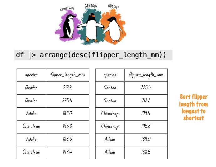
  rename(opioid_pills = number_pills)

The arrange() function

Artwork by @allison_horst

The arrange() function will sort a data frame by a variable or set of variables. Let’s filter to choose only CO counties in 2010 and sort by number of pills purchased per person. We can do this with a pipe:³

opioid_counties |> 
  filter(year == 2010 & state == "CO") |> 
  arrange(pills_per_capita) 

The default for arrange() is to sort the mentioned variables in ascending order. If instead you wanted to sort from high to low (i.e, descending order), then you may use the desc() function as an argument to arrange():

opioid_counties |> 
  filter(year == 2010 & state == "CO") |> 
  arrange(desc(pills_per_capita)) 

Now that we’ve created a new data frame, let’s use it to make a bar chart — with counties on the y-axis and pills per capita on the x-axis. To make the bars appear in order from lowest to highest (or highest to lowest) based on pills per capita, we need to reorder the county variable. We can do this using the fct_reorder() function from the forcats package.

Instead of writing y = county, we’ll write: y = fct_reorder(county, pills_per_capita).

The function takes two arguments:

1. The factor you want to reorder — in this case, county

2. The variable to order by — here, pills_per_capita.

This ensures the counties appear in a meaningful order in the plot.

opioid_counties |> 
  filter(year == 2010 & state == "CO") |> 
  ggplot(mapping = aes(x = pills_per_capita, y = fct_reorder(county, pills_per_capita))) +
  geom_col(fill = "#E24E42") +
  labs(title = "Number of pills purchased per capita in 2010 by county in CO",
       x = "Number of pills per capita",
       y = "",
       caption = "Source: The Washington Post, ARCOS") +
  theme_minimal()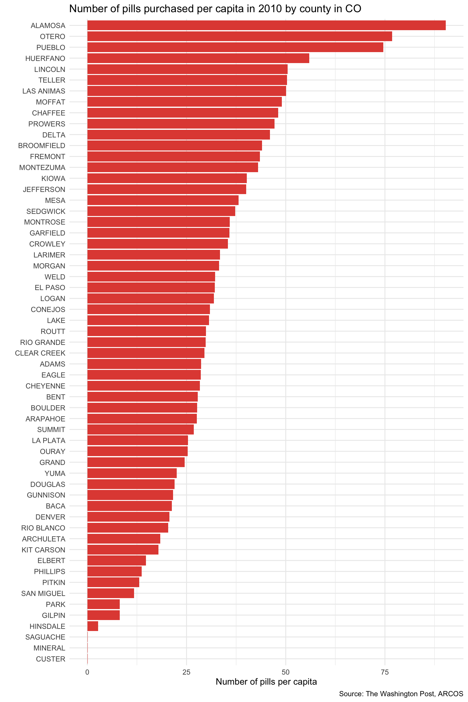

Pivot data with tidyr

Artwork by @allison_horst

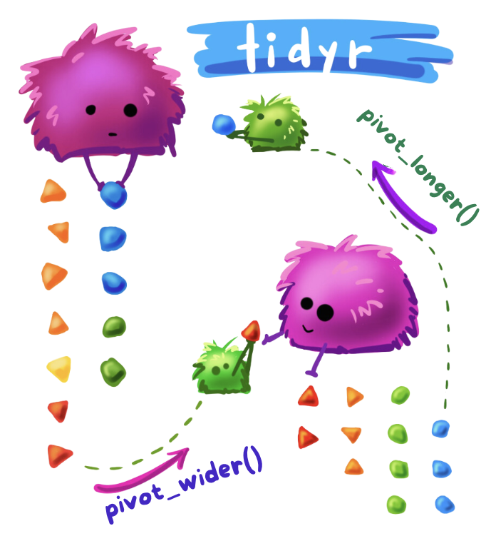
pivot_wider and pivot_longer are functions from the tidyr package for reshaping data. The pivot_longer() function pivots data from a wide format to a long format, while the pivot_wider() function pivots data from a long format to a wide format.

Pivot from long to wide

pivot_wider() is used to make a data frame wider by increasing the number of columns and decreasing the number of rows. Essentially, it converts rows into columns. This is useful when you have data in a “long” format and you want to make it “wide” for a different kind of analysis or visualization.

The basic syntax of the pivot_wider() function is:

pivot_wider(id_cols, names_from, values_from, names_prefix)

• id_cols: A set of columns that uniquely identify each observation.
• names_from: The name of the column in the original data frame that contains the names for the new columns.
• values_from: The name of the column that contains the values to be placed in the new columns.
• names_prefix: A string added to the start of every variable name.

In the opioid data frame, there are up to 9 rows of data per county — one row for each year available (2006 to 2014). Let’s take a look at a subset of the data frame that has the unique identifiers (fips, county, state), as well as year and pills_per_capita.

opioid_counties |> 
  select(fips, county, state, year, pills_per_capita) |> 
  head(n = 18)

Imagine that we’d instead like to pivot or reshape the data frame so that each county has a single row of data (rather than 9 rows of data), and that rather than one variable for pills_per_capita which is indexed by year, we would like to have one column that represents pills_per_capita for each year. We can use pivot_wider() to accomplish this task.

opioid_counties_wide <-
  opioid_counties |> 
  select(fips, county, state, year, pills_per_capita) |> 
  pivot_wider(id_cols = c(fips, county, state),
              names_from = year, 
              values_from = pills_per_capita, 
              names_prefix = "pills_per_capita_in_")

opioid_counties_wide |> 
  head()

Let’s break down the code:

• The argument id_cols lists the ID variables that uniquely identify each county.

• The argument names_from = year specifies that the new columns’ names should be based on the values in the year column (i.e., a variable in the data frame — the one that indexes the rows of data for each county).

• The argument values_from = pills_per_capita specifies that the values in the new columns should come from the pills_per_capita column.

• Finally, names_prefix = "pills_per_capita_in_" indicates that we’d like to add a prefix to the new column names. For example, for year 2010, there should be a new column named pills_per_capita_in_2010 that denotes the pills per capita values for the year 2010. If we left off this argument, the column names would be the year — e.g., just 2010 rather than pills_per_capita_in_2010. A number is not a suitable name for a variable — therefore, when the index row of the long data frame (i.e., the variable identified in the names_from argument) is a number, then making use of the names_prefix argument is advised.

To be sure we understand what’s happening, let’s take a look at the original data frame and the reshaped data frame for one county — Larimer County in Colorado.

Here’s what the relevant variables in the data frame looked like to begin with:

Once reshaped using pivot_wider(), the data for Larimer county in the pivoted data frame (opioid_counties_wide) looks like this:

Important

Take a moment to match up the pills per capita scores for each year across the two versions of the data frame to see that the values are identical (you’ll need to arrow over in the wide data frame to see all of the years). Indeed, they are the same, it’s just that one is in a long format and one is in a wide format.

Pivot from wide to long

pivot_longer() is used to make a data frame longer by increasing the number of rows and decreasing the number of columns. Essentially, it converts columns into rows. This is particularly useful when you have data in a “wide” format and you want to make it “long” for analysis or visualization.

The basic syntax of the pivot_longer() function is:

pivot_longer(cols, names_to = "name", values_to = "value")

• cols: The columns you want to convert into rows.
• names_to: The name of the column that will store the old column names.
• values_to: The name of the column that will store the values previously in the specified columns.

To demonstrate, let’s put the opioid_counties_wide data frame back into a long data frame format (i.e., reverse what we initially accomplished with pivot_wider()).

opioid_counties_long <-
  opioid_counties_wide |> 
  pivot_longer(cols = starts_with("pills_per_capita"), 
               names_to = "which_year", 
               values_to = "pills_per_capita")

opioid_counties_long |> 
  head()

With the pivot_longer() function, we want to gather all of those year-specific columns into two columns:

• One called which_year that stores the original column names (e.g., “pills_per_capita_2006”).

• One called pills_per_capita that stores the actual values from those columns.

The result is a longer data frame where each row now represents a single county-year combination, instead of having one row per county with many year-specific columns.

In looking at the output, we see that we’re back to a long data frame — with up to 9 rows of data per county — one for each year.

You might notice here that the which_year variable looks different than year in the original data frame. This is because, pivot_longer() uses the names of the wide variables for the assigned index values (i.e., pills_per_capita_in_2010 rather than just 2010). We can fix this up with a couple of extra steps.

The separate() function splits the values in a column into one or more columns. Here, we ask R to separate the variable which_year into two columns — one called prefix and one called year. The sep = argument indicates where in the string the separation should occur. For the string “pills_per_capita_in_2010”, we request the separation at the point of “in” in the string. Therefore this string will be broken into two — one that is recorded in the variable called prefix and will simply contain the string pills_per_capita, and one that is recorded in the variable called year and will contain the actual year. Take a look at the result below.

opioid_counties_long |> 
  separate(which_year, into = c("prefix", "year"), sep = "_in_") |> 
  head()

This looks good — but, there are a some additional fixes that we can apply to restore the data frame to it’s original form. First, notice that the variable year in the above data frame is a character (noted by <chr> below the variable name). We want it to be recognized as an integer (<int>) (as it was in the original data frame). We can accomplish this goal by mutating year with the as.integer() function — which forces a variable to be treated as an integer. Second, the variable called prefix is useless here — as it just stores the string “pills_per_capita”. We can remove it with the select() function (if you put a minus sign (-) in front of a variable name, it does the opposite of the usual select() behavior — it removes that variable from the data frame). Let’s redo the code adding these two steps.

opioid_counties_long <-
  opioid_counties_long |> 
  separate(which_year, into = c("prefix", "year"), sep = "_in_") |> 
  mutate(year = as.integer(year)) |> 
  select(-prefix)

opioid_counties_long |> 
  head()

Tip

If efficiency is your thing — you could actually perform the separation of the prefix from the year right inside of the pivot_longer() function. If you’re curious — please see the code below for an equivalent example:

opioid_counties_long <-
  opioid_counties_wide |> 
  pivot_longer(cols = starts_with("pills_per_capita"), 
               names_to = c("prefix", "year"), 
               names_sep = "_in_",
               values_to = "pills_per_capita") |> 
  mutate(year = as.integer(year)) |> 
  select(-prefix)

opioid_counties_long |> 
  head()

The left_join() function

Awesome gif created by Garrick Aden-Buie

The joining dplyr functions are used to merge (i.e., join) two data frames together.

Before doing so, let’s pause to introduce the left_join() syntax. left_join() is a function used to combine two data frames based on a common column or variable. It is called a “left join” because it takes all the rows from the left data frame and matches them with corresponding rows from the right data frame.

Imagine you have two data frames, let’s call them df_a and df_b. Each data frame has multiple columns, but they share one column that contains similar information, such as an ID. A left join allows you to combine these two data frames based on that shared column. This shared column is often referred to as a key.

The code to combine these two data frames is:

new_df <-
  df_a |> 
  left_join(df_b, by = "ID")

The code snippet above performs a left join operation to merge two data frames, df_a and df_b, based on a common column ID. The resulting merged data frame is stored in a new object called new_df.

When you perform a left join, the resulting data frame will include all the rows from the first (i.e., left) data frame (that is df_a), along with the corresponding matching rows from the second (i.e., right) data frame (that is df_b). If there are no matches in df_b for a particular row in df_a, the values from df_b will be filled with missing values (i.e., NA).

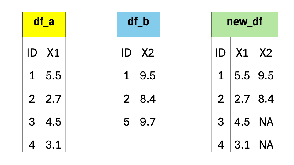
In simple terms, a left join takes the left data frame as the primary reference and combines it with matching rows from the right data frame. It ensures that all the information from the left data frame is included, while also bringing in relevant information from the right data frame if available.

For an applied example, we might be interested in examining correlates of opioid pills per capita in the counties. Data based on census records often provides rich and interesting data to describe geographic units — like counties. Let’s read in another county-level data frame, called county_info.Rds, that includes the Area Deprivation Index (adi) for each county in 2010, as well as the percent of residents in the county who were non-Hispanic White based on 2010 census records (white_non_hispanic_pct2010). The Area Deprivaition Index is a measure created by the Health Resources & Services Administration (HRSA) using US Census records, and serves as a measure of concentrated socio-economic disadvantage in the county.

In this example, we’ll use the following variables from the county_info.Rds data frame:

Variable	Description
fips	A 5 digit code that identifies each county
adi	The area deprivation index — a higher score means more deprivation
white_non_hispanic_pct2010	The percent of county residents who identify as non-Hispanic White

Let’s import the data frame and select just the variables we will use.

county_info <- read_rds(here("data", "county_info.Rds")) |> 
  select(fips, adi, white_non_hispanic_pct2010)

county_info |> 
  head()

Let’s now merge (i.e., join) the county_info data frame with the wide version of the opioid_counties data frame that we created in the last section on reshaping data — recall that the wide data frame is called opioid_counties_wide. Since fips is in both data frames, and it uniquely identifies each county, we can join the data frames together using fips as the matching variable.

In the code below a new data frame called opioid_merged is created that begins with the initial data frame (i.e., the left data frame – opioid_counties_wide) and then joins in the county_info data frame. The variable fips is used to match the rows of data together.

opioid_merged <-
  opioid_counties_wide |> left_join(county_info, by = "fips") 

opioid_merged |> 
  select(fips, county, state, adi, white_non_hispanic_pct2010, everything()) |> 
  head()

Tip

I use a left_join() merge most often in practice; however, there are many different types of joins available, and the best choice depends on the qualities of the data frames to be joined and the analyst’s needs.

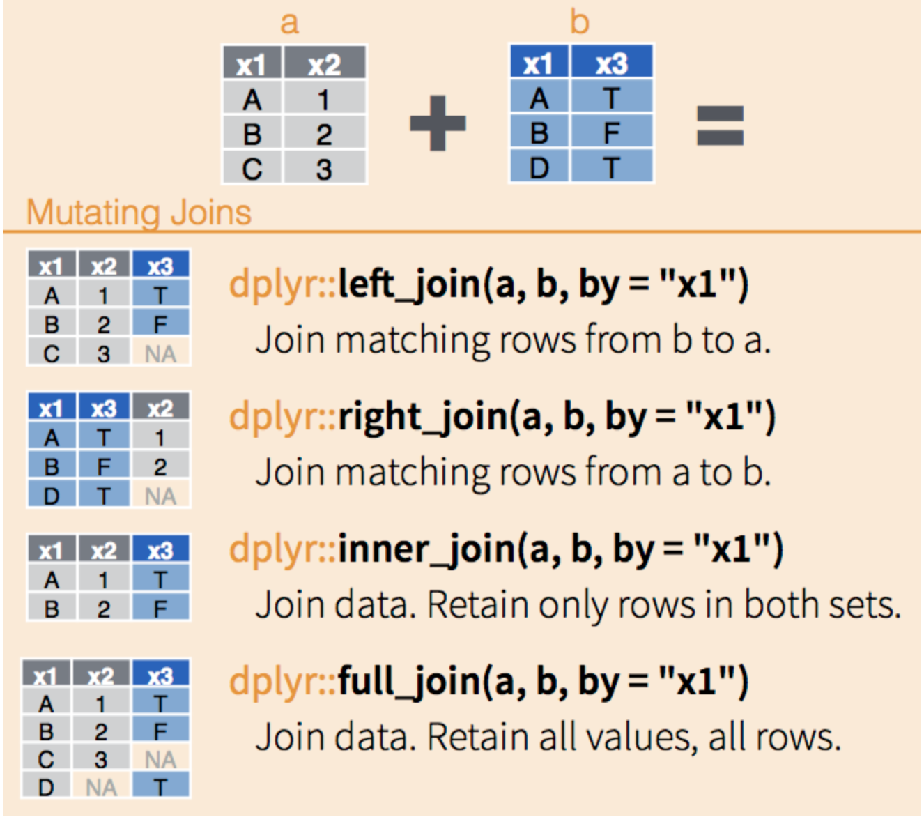
• left_join() keeps all the entries that are present in the left (first) data frame and includes matching entries from the right data frame. If there are no matching entries in the right data frame, the result will contain NA for columns from the right data frame.

• right_join() keeps all the entries that are present in the right data frame and includes matching entries from the left data frame. If there are no matching entries in the left data frame, the result will contain NA for columns from the left data frame.

• inner_join() keeps only the entries that are present in both data frames. This type of join returns only the entries where the key(s) exist in both data frames, effectively filtering out non-matching rows from either side. It does not generate any NA values because all returned rows have matching information from both data frames.

• full_join() keeps all of the entries in both data frames, regardless of whether or not they appear in the other data frame. Non-matching entries in either data frame will result in NA values for the missing columns from the other data frame.

You can explore these other join types here and view other cool gifs to visualize these join types here.

The case_when() function

Artwork by @allison_horst

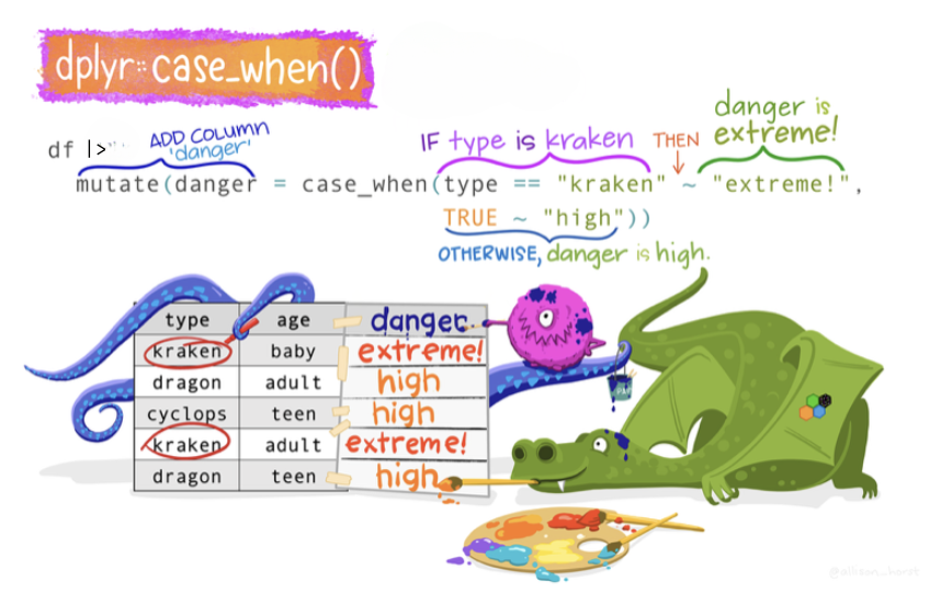
The case_when() function allows you to construct a new variable by specifying a set of conditions and corresponding values based on the data in existing variables. It works similarly to a series of if-else statements, allowing for more readable and concise code. For each observation (row) in your data frame, case_when() evaluates the conditions in the order they are specified, and assigns the value associated with the first condition that is met. If none of the conditions are met, it assigns NA (R’s missing data indicator) to that observation in the new variable.

We can think of case_when() like a decision-making robot in a game. This robot has a list of rules and gives you prizes based on these rules. It goes through the rules one by one, and as soon as it finds a rule that you meet, it gives you the prize for that rule and stops. If none of the rules are met, you don’t get a prize.

Here’s an example. Imagine you are playing a game where you earn points, and at the end, you get a badge based on how many points you earned:

• If you earn less than 10 points, you get the “Bronze” badge.
• If you earn 10 to 19 points, you get the “Silver” badge.
• If you earn 20 or more points, you get the “Gold” badge.

Now, let’s use our robot (case_when()) to give badges based on points. We can tell the robot the rules and prizes like this:

badge = case_when(
  points < 10 ~ "Bronze", 
  points < 20 ~ "Silver", 
  points >= 20 ~ "Gold")

Here’s what this code tells the robot:

• Look at the points.
• If points are less than 10, the prize is “Bronze”. (The robot stops here if this rule is met.)
• If points are less than 20, the prize is “Silver”. (Again, the robot stops if this rule is met.)⁴
• If points are 20 or more points, the prize is “Gold”.

Let’s use the opioid_merged data frame that we just created to see an example of case_when() in action. For this example, we will create a new variable called county_raceeth which will be coded “white county” if white_non_hispanic_pct2010 is greater than or equal to 50% (i.e., half or more of the residents identify as non-Hispanic white) and “minority county” if fewer than half of the residents identify as non-Hispanic White.

Using the opioid_merged data frame, we’ll use the case_when() function to create our new variable county_raceeth. To reiterate, each case_when() statement has two parts — the part before the tilde (~) and the part after the tilde. The part before the tilde is called the left hand side (LHS) and the part after the tilde is called the right hand side (RHS). case_when() uses the LHS part of the statement as the condition to test for and the RHS as the value to return. case_when() works in sequence through the conditions, finding when the LHS is true for each case (i.e., row of data), and then returning the value associated with that condition.

Each row in the data frame will be evaluated, if white_non_hispanic_pct2010 is < 50, then “minority county” will be recorded for county_raceeth. The second case_when() statement is only evaluated if the first case_when() statement is false. In the second case_when() statement, if white_non_hispanic_pct2010 is >= 50, then “white county” will be recorded for county_raceeth. Any rows that don’t match any of the conditions will be assigned NA (NA is R’s missing data indicator) for county_raceeth.

opioid_merged <-
  opioid_merged |> 
  mutate(county_raceeth = case_when(white_non_hispanic_pct2010 < 50 ~ "minority county", 
                               white_non_hispanic_pct2010 >= 50 ~ "white county")) |>
  select(fips, adi, white_non_hispanic_pct2010, county_raceeth, pills_per_capita_in_2010)

opioid_merged |> 
  head(n = 30)

Practice Wrangling and Plotting

With these data compiled, let’s take the opportunity to determine if counties with more socio-economic disadvantage had more pills coming into their communities. This is an important public health question. The socio-economic vitality of a community plays an important role in promoting health, well-being, and prosperity for residents. As such, public health scientists recognize socio-economic advantage vs. disadvantage, of both an individual and their community, as a key social determinant of health. Healthy People 2030, a public health effort coordinated by the Office of Disease Prevention and Health Promotion (ODPHP), defines social determinants of health and describes their importance:

Social determinants of health are conditions in the environments in which people are born, live, learn, work, play, worship, and age that affect a wide range of health, functioning, and quality-of-life outcomes and risks. Conditions (e.g., social, economic, and physical) in these various environments and settings (e.g., school, church, workplace, and neighborhood) have been referred to as “place.” In addition to the more material attributes of “place,” the patterns of social engagement and sense of security and well-being are also affected by where people live. Resources that enhance quality of life can have a significant influence on population health outcomes. Examples of these resources include safe and affordable housing, access to education, public safety, availability of healthy foods, local emergency/health services, and environments free of life-threatening toxins. Understanding the relationship between how population groups experience “place” and the impact of “place” on health is fundamental to the social determinants of health—including both social and physical determinants.

Let’s use our data to take a look at the relationship between the area deprivation index (adi) and number of pills per capita purchased (pills_per_capita_in_2010). Given that the opioid pandemic was especially wide spread in predominantly non-Hispanic White communities during the initial years, we will facet our scatterplot by the country_raceeth indicator created earlier.

Create a scatter plot

opioid_merged |> 
  select(adi, pills_per_capita_in_2010, county_raceeth) |> 
  drop_na() |> 
  ggplot(mapping = aes(x = adi, y = pills_per_capita_in_2010)) +
  geom_jitter(color = "dark gray") + 
  geom_smooth(method = "loess", se = FALSE, formula = y~x) +
  facet_wrap(~county_raceeth) +
  theme_bw() +
  labs(title = "Is county-level socio-economic disadvantage associated with more opioid pills per capita?",
       x = "Area Deprivation Index",
       y = "Opioid pills per capita")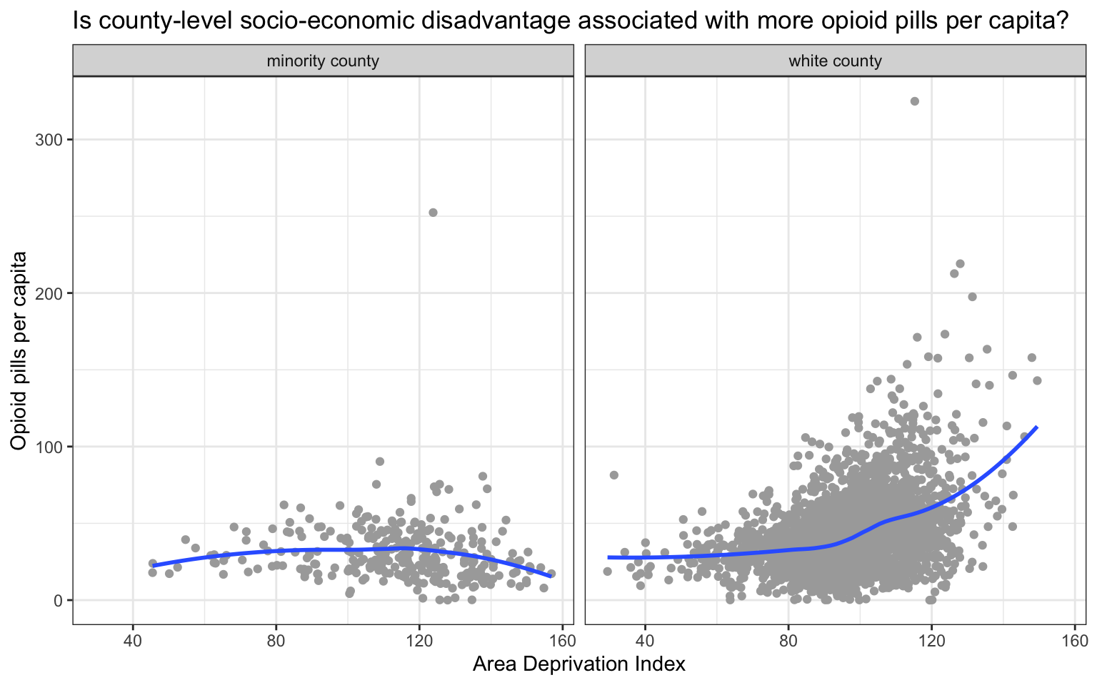

Among predominantly White counties, we see evidence that greater socio-economic disadvantage was associated with more pills per capita. Interestingly this trend is not apparent in predominantly minority communities. In other words, our graph suggests that in 2010, during the height of the time when opioid pills were flooding into American communities, the most pills were being directed to pharmacies in the most socio-economically disadvantaged (predominantly) White communities. If you’d like to read more about the marketing strategies used by Purdue Pharma to boost sales of OxyContin, please listen to this story by National Public Radio.

Importing and Exporting Data in R

Let’s wrap up this Module by learning how to import (read in) and export (write out) data files.

Import data

Import R data frame

So far in this course, we have imported R data frames.

county_info <- 
  read_rds(here("data", "county_info.Rds"))

But, you can import many different types of data frames to use in R. Commonly, data is entered in excel and saved as a comma delimited file (.csv file extension). If the adi_counties data frame we used in this Module were a csv file — called adi_counties.csv. We could import it using the read_csv() function, which is part of the tidyverse.

Import a csv file

county_info <- 
  read_csv(here("data", "county_info.csv")) 

Or, if the data frame were stored as an excel file (.xlsx), we could use the readxl package’s read_excel() function. Though readxl is part of the tidyverse, it’s not automatically loaded — so the library needs to be loaded before using it (see the double colon operator in the code below):

Import a excel file

county_info <- 
  readxl::read_excel(here("data", "county_info.xlsx")) 

The readxl package has many features that can be used to read in “tricky” excel files (e.g., multiple sheets, need for skipping rows, range specifications, etc.).

Import other types of files

The haven package, which is part of the tidyverse, allows for the import of many different types of data frames — like SPSS, SAS, and much more. If you encounter these types of data files, you can explore the haven package on your own.

Export data

Sometimes, we may want to save a new version of our data frame. For example, let’s imagine that we want to save the opioid_merged data frame that we used in the last section. We can do this with the following code that makes use of the write_rds() function (to save as a R data file) or the write_csv() function (to save as a csv file). Notice the use of the here() function so the data is directed to be saved in our data folder. You should never overwrite the original data file though — if you make changes to the source (i.e., original) data file — it’s important to save it with a different name so that the original file remains intact.

Export a Rds file

opioid_merged |> 
  write_rds(here("data", "opioid_merged_updated.Rds"))

Export a csv file

opioid_merged |> 
  write_csv(here("data", "opioid_merged_updated.csv"))

Export a xlsx file

opioid_merged |> 
  writexl::write_xlsx(here("data", "county_info.xlsx"))

Export other types of files

Using the haven package mentioned above, you can write out a data frame to any other type. For example, to save your R data frame as a SPSS data frame.

Learning Check

After completing this Module, you should be able to answer:

1. What is data wrangling, and why is it a critical first step in data analysis?
2. What is the role of dplyr in a tidyverse workflow?
3. How does filter() help you isolate specific observations in a dataset?
4. How does mutate() support the creation or transformation of variables?
5. How do you use arrange() to reorder rows based on values in one or more variables?
6. How do group_by() and summarize() work together to produce summaries by group?
7. How does case_when() help you recode or classify values based on multiple conditions?
8. How do you import a dataset into R using read_csv(), and how do you export it using write_csv()?
9. What is the pipe operator (|>), and how does it help you build readable, modular code?
10. What does it mean to say that tidyverse functions follow a “data in, data out” logic?

Resources

• The incredible book, R for Data Science, is truly the authority on all things related to data wrangling with R.

Footnotes

1. A Boolean operator is a word or symbol used in logic and computer science to create expressions that can evaluate to true or false. Boolean operators are fundamental to forming logical statements and are used extensively in programming, database searches, and search engines.

2. A vector is an ordered collection of elements of the same data type. It is a one-dimensional array that can hold values such as numbers, characters, logical values, or other R objects. Since all three elements in this example are numbers — 2010, 2012, 2014 — then it is classified as a vector.

3. In R, a pipe is a tool used to make code more readable and expressive by connecting a sequence of operations. The pipe operator is written as |> (or %>% in older code). It takes the result from the left-hand side and passes it as the first argument to the function on the right-hand side.

4. In the case_when() function, conditions are evaluated sequentially, and the first true condition determines the outcome. This means that once a condition is met, no further conditions are checked. In the example above, we first check if points < 10 for the “Bronze” badge. Since this condition catches all points less than 10, the next rule, points < 20, only applies to points that are between 10 and 19 (inclusive). This is why we don’t need to explicitly check for points >= 10 & points < 20. The final rule, points >= 20, only applies to points 20 or more.