Basic Rules of Probability

Module 5

Learning Objectives

By the end of this Module, you should be able to:

• Define probability as a measure of uncertainty ranging from 0 (impossible) to 1 (certain)
• Distinguish between theoretical and empirical probability and describe when each is appropriate
• Define a data generating process (DGP)
• Apply the addition rule of probability for mutually exclusive and non-mutually exclusive events
• Apply the multiplication rule of probability for independent and dependent events
• Calculate marginal, joint, and conditional probabilities using a contingency table
• Define and calculate sensitivity, specificity, and positive predictive value (PPV) from cross-tabulated data
• Apply Bayes’ Theorem to update probabilities given new evidence

Overview

Probability is the language we use to describe uncertainty — and in statistics, uncertainty is everywhere. Whether we’re estimating how many people support a policy, predicting whether a treatment will work, or testing if a coin is fair, we rely on probability to guide our thinking. This Module introduces the basic ideas of probability and how they form the foundation of statistical reasoning.

Let’s begin our exploration of probability with this short video from Crash Course Statistics:

What is probability?

Probability is a way to put a number on how likely something is to happen. It ranges from 0 to 1: a probability of 0 means the event can’t happen at all (like rolling a 7 on a six-sided die), and a probability of 1 means it’s guaranteed to happen (like the sun rising tomorrow). For example, if you flip a fair coin, the chance of it landing on heads is 0.5, or 50% — it’s equally likely to land on heads or tails.

Why is probability important for statistics?

At its core, statistics is about making sense of data — especially when things are uncertain. And that’s where probability comes in.

Probability helps us reason under uncertainty. It gives us a way to say how likely something is, even when we don’t know for sure. In statistics, we often look at a small set of data and try to figure out what’s going on in the bigger picture — or what might happen next. Probability is the tool that lets us do that.

Let’s say you survey a group of students and find that 60% say they’re stressed about school. Can you use that number to say something about all students? What if you repeated the survey and got 55% next time? Or 65%? Probability helps us understand how much these numbers might vary, and how confident we can be in the conclusions we draw.

But probability isn’t just about estimating a proportion — it shows up everywhere in statistics:

1. Modeling Uncertainty: Imagine you give the same cold medicine to 100 people. Some get better quickly, some slowly, and a few don’t improve at all. This variation is expected — and probability helps us describe it. We can’t predict exactly who will respond how, but we can use probability to model the range of likely outcomes. It gives us a way to say, for example, “Most people improve within 3 days, but about 10% might take a week or more.

2. Inferential Statistics: Imagine you’re testing a new therapy for depression and find that, in your sample of 50 clients, the average depression score is 6.2. But your real question is: What’s the average score we’d expect if we gave this therapy to all clients with depression? Probability helps you estimate how close your sample mean is to the true population mean. It gives you a way to say, “We’re pretty confident the average depression score for all clients would fall within this range.”

3. Hypothesis Testing: Suppose you’re running a memory experiment to test whether a new strategy helps people recall more words. You compare two groups — one using the strategy, one not. If both groups truly have the same memory ability, how likely is it that you’d still see a difference as big as the one in your data? That’s a probability question. It helps you decide whether the observed difference is likely just due to chance — or whether the strategy actually made a difference.

4. Bayesian Statistics: Suppose you’re studying how stress affects heart health. Based on past research, you believe that high stress levels increase the risk of high blood pressure. That’s your starting belief, or prior. As you collect new data from a workplace stress intervention, you use probability to update that belief — maybe the data suggest the effect is smaller (or larger) than you thought. In Bayesian statistics, probability helps you refine your understanding of the process that generated the data as new evidence becomes available.

5. Predictive Modeling: Suppose you’re trying to predict which job applicants are most likely to succeed in a sales role. You collect data on things like interview scores, personality traits, and prior experience. Then you build a model to estimate how likely each candidate is to meet future sales targets. Probability helps you assign those likelihoods — not as guarantees, but as informed estimates — based on patterns learned from past data. It’s a way of modeling the process that produces success and using that model to guide hiring decisions.

6. Study Design: Even before collecting data, probability helps us plan. How large should our sample be to detect an effect if one exists? What’s the risk of missing a real difference just by chance? These kinds of questions — about how confident we can be in our results — are all grounded in probability.

So why does this all matter?

Because probability is what connects the data we observe to the process that produced it — what we call the data generating process (or DGP). The DGP includes the causes, conditions, and randomness that shape real-world outcomes. Learning to understand this connection — how data arise from an underlying process — is at the heart of statistical thinking. Probability gives us the tools to reason about that process, even when we can’t see it directly.

What is a Data Generating Process?

In this course, we’ll talk a lot about the data generating process, or DGP. That’s just our term for the system — the causes, conditions, and randomness — that produces the data we observe.

A simple metaphor: Baking cookies

Imagine you just pulled a tray of cookies from the oven. Those cookies are like your data. But they didn’t appear out of nowhere. They were produced by a process: the recipe, the ingredients, the baking time, the oven temperature — and maybe a little randomness (like uneven chocolate chip distribution).

The DGP is everything behind the scenes that shaped the final result. In statistics, we do the same thing: we look at data and ask, “What process produced this?”

And just like in baking, if we want to understand why the cookies turned out the way they did — or how to make better ones next time — we can’t just focus on one piece, like the oven temperature. We have to think about the whole process.

Examples of DGPs in Psychology

Cognitive Neuroscience

Let’s say you’re studying working memory using fMRI. You show participants letter sequences and ask them to recall them while measuring brain activity.

Your data might be the BOLD signal from a specific brain region.

The DGP includes:

• Participant factors (age, attention, baseline brain activity)
• Task features (stimulus timing, memory load)
• Environmental factors (scanner noise, temperature)
• Measurement error and chance

The BOLD signal isn’t the whole story — it’s an output from a complex process you’re trying to understand.

Industrial-Organizational Psychology

Suppose you’re studying employee performance using annual ratings.

You don’t see everything that affects performance — like motivation, job stress, or team climate — but you do have some related information, like:

• Hours worked per week
• Self-reported job satisfaction
• Supervisor evaluations
• Number of sick days taken

These are observable pieces of a much bigger process — the data generating process (DGP) — that leads to performance ratings.

Using statistics, you can explore patterns in the data to make inferences about that process. For example:

• If employees who report high job satisfaction also tend to get better performance ratings, that suggests satisfaction might be part of the DGP.
• If people with high stress scores are consistently rated lower, stress might be another factor.

You’re not seeing the full DGP — but by examining how different variables relate to the outcome, you can start to understand which parts of the process matter most. That’s how we learn about the DGP from the data we do have.

Why it matters

Researchers aren’t just interested in what happened — we want to know why it happened. That means understanding the process that produced the data.

We usually can’t see the full DGP directly. But using probability and statistics, we can reason backward from the data and make informed guesses about how the process works.

This is how we go from describing data to explaining it — and why statistical reasoning is so powerful.

The critical importance of the DGP

Carefully considering the DGP is essential — not just after data collection, but from the very beginning of your study.

The DGP is the full system that produces the data: the underlying causes, conditions, and random factors at play. If you focus only on the specific variables you plan to measure, you risk missing important parts of the bigger picture.

When you think broadly about the DGP — before you collect or analyze data — you can:

• Design more meaningful and valid studies
• Identify which variables are most relevant and informative
• Anticipate sources of noise, bias, or confounding
• Make more accurate and cautious interpretations of your results

Good statistical reasoning starts with a deep question:
What process am I trying to understand, and how can I best observe it?

By grounding your research in the full context of the DGP, you’re more likely to produce insights that are accurate, generalizable, and useful.

Probability vs. Statistics: What’s the difference?

Once you understand the idea of a DGP, the difference between probability and statistics becomes much clearer:

• Probability starts with the process and asks:
  What kind of data should we expect?
  (If a coin is fair, there’s a 50% chance of heads.)

• Statistics starts with the data and asks:
  What can we learn about the process?
  (If a coin lands heads 75 out of 100 times, maybe it’s not fair.)

Think of it this way:

• Probability = Start with the DGP → Predict the data
  
• Statistics = Start with the data → Learn about the DGP

Why this matters to you

Understanding the DGP — and how probability and statistics relate to it — helps you see what you’re really doing when you analyze data:

• In research, we use data to test our theories. If a health campaign claims to reduce smoking, we collect data and ask: Did behavior change in a way that fits with the theory?
• Most of the time, we don’t know the complete DGP in advance. Statistics helps us figure it out.
• Real-world data is messy and variable. Probability helps us understand what patterns are meaningful and what might just be noise.
• As we collect more data, we refine our understanding of the DGP — and get closer to the truth.

Why you need probability to learn statistics

Even though statistics focuses on analyzing data, it’s built on the foundation of probability.

To learn statistics, you need to understand:

• What randomness means
• What it means for something to be likely or unlikely
• How sample data can vary even when drawn from the same DGP

These ideas will show up all semester. Probability is what lets you reason clearly about uncertainty — so you can use data to learn about the world and the processes that shape it.

Defining Events and Understanding Probability

Probability gives us a way to describe uncertainty using numbers between 0 and 1. An event is something we’re interested in — like flipping heads on a coin, drawing a heart from a deck, or having type O blood. In probability theory, we define events formally so we can assign and calculate probabilities.

An event can be:

• A single outcome, like rolling a 6 on a die
  
• A set of outcomes, like rolling an even number (2, 4, or 6)
  
• Or a more complex condition, like drawing a face card or a heart from a deck

We use notation like \(P(A)\) to represent the probability of event A occurring.

Elementary events and the sample space

An elementary event is a single outcome that can’t be broken down further. The sample space is the set of all possible outcomes. For example, the ABO blood type system has four elementary events:

• A
  
• B
  
• AB
  
• O

These make up the sample space of possible blood types. Suppose large population studies have found:

• \(P(\text{A}) = 0.42\)
  
• \(P(\text{B}) = 0.10\)
  
• \(P(\text{AB}) = 0.04\)
  
• \(P(\text{O}) = 0.44\)

These values are probabilities — and they must always add up to 1, because the sample space includes all possible outcomes. This is known as the law of total probability:

\[ P(\text{A}) + P(\text{B}) + P(\text{AB}) + P(\text{O}) = 1.0 \]

Two ways to calculate probability

We can estimate probabilities in two ways: theoretically and empirically.

Theoretical Probability

This kind of probability is based on logic and assumptions about the underlying situation. For example, in a standard deck of cards:

\[ P(\text{Heart}) = \frac{13}{52} = 0.25 \]

This assumes all outcomes are equally likely and the system is perfectly random — no bias, no errors.

Empirical Probability

This type is based on real-world data. Suppose we survey 300 teens and 225 say they use social media:

\[ P(\text{Using social media}) = \frac{225}{300} = 0.75 \]

This gives us an observed or empirical probability based on the data we collected.

Why distinguish between theoretical and empirical?

• Theoretical probability is idealized — it helps us make predictions, design studies, or simulate outcomes.
• Empirical probability is grounded in reality — it tells us what’s actually happening in a specific context.

By comparing the two, we can assess how well our models match the real world.

Bringing it all together: Simulation

Simulation is one way that we can bridge theory and real-world observation.

It allows us to take what we know — such as population probabilities — and explore what we might see in practice. For example, suppose we know that 44% of people have type O blood. What happens if we randomly sample 1,000 people? Will exactly 44% have type O blood? Probably not.

That’s where simulation comes in.

Why learn simulation? Because it makes abstract ideas concrete

Let’s say we want to understand how common type O blood is. We know the population probability is 0.44 — but in a real-world sample of 1,000 people, that number will fluctuate. One sample might show 42% with type O, another 46%, and another might hit 44% exactly.

Simulation lets us “try it out” — again and again. Each simulated sample helps us see how random variation works in action. Over time, we start to build intuition around key ideas, such as:

• Why samples differ even when drawn from the same population
• What range of results is “typical” or expected
• How much confidence we can have in our conclusions from one sample

In short, simulation helps you think like a data scientist. It trains you to expect variation, question your assumptions, and understand what kinds of results are meaningful — and which ones might just be due to chance.

Here’s how we’d conduct a simulation for this simple example of ABO blood type using R:

library(tidyverse)

set.seed(1122334455)

blood_types_df <- tibble(
  blood_type = sample(
    x = c("A", "B", "AB", "O"),
    size = 1000,
    replace = TRUE,
    prob = c(0.42, 0.10, 0.04, 0.44)
  )
)

blood_types_df |> 
  count(blood_type) |> 
  mutate(proportion = n / sum(n))

Let’s break down the parts of this code:

1. set.seed(): This function ensures reproducibility. While it’s not required, it’s helpful when you want to get the same results every time you run the code — which is especially useful when sharing code with others or teaching. Without it, the proportions of each blood type in your sample would still be based on the same probabilities, but the exact results would fluctuate due to random variation.

2. Creating a Data Frame (tibble()): The tibble() function is used to create a data frame. Here, a data frame called blood_types_df is created with one variable named blood_type.

3. Sampling (sample()): The sample() function is used to generate random samples. In this context, it’s used to simulate the blood types of 1000 people. Let’s look at the arguments passed to this function:

   • x = c(“A”, “B”, “AB”, “O”): This is the vector of possible outcomes or categories from which samples are drawn. Here, it represents the four blood types.

   • size = 1000: This specifies the number of samples to draw, which is 1000 in this case. It means we’re simulating the blood types for 1000 individuals.

   • replace = TRUE: This indicates that sampling is done with replacement. In other words, once a blood type is selected for an individual, it’s not removed from the pool of options for the next individual. This makes sense here since an individual’s blood type doesn’t affect another’s.

   • prob = c(0.42, 0.10, 0.04, 0.44): This vector provides the probabilities associated with each category in x. These values must sum to 1, representing a complete probability space for the blood types. The probabilities correspond to the likelihood of each blood type in the population.

This simulated sample lets us see probability in action and compare our results to both theoretical and empirical expectations. For example, we can calculate the proportion of people with each blood type. The count() function calculates the number of cases in the simulated data that have each blood type, then the mutate() function is used to turn the counts into proportions. Here, the proportion of people with each blood type should be close to the probabilities that we supplied for the simulation.

blood_types_df |> 
  count(blood_type) |> 
  mutate(proportion = n / sum(n))

Basic Rules of Probability

The basic rules of probability help us to understand and calculate the likelihood of various events in a consistent and reliable manner.

Addition rule of probability

The addition rule helps us figure out the probability that at least one of two events will happen. In other words, it helps answer questions like:

“What’s the chance that event Y or event Z happens?”

In probability, this is called the union of two events and is written as:

\[ P(Y \text{ or } Z) = P(Y \cup Z) \]

There are two situations to consider: when events are mutually exclusive and when they are not mutually exclusive.

When events are mutually exclusive

Two events are mutually exclusive if they can’t happen at the same time. If one happens, the other can’t.

In that case, the probability of either happening is just the sum of their individual probabilities:

\[ P(Y \text{ or } Z) = P(Y) + P(Z) \]

Example:
Each person has exactly one ABO blood type — A, B, AB, or O — so these types are mutually exclusive.

Let’s say we want to know the probability that a person has Type A or Type AB blood. From population data:

• \(P(\text{Type A}) = 0.42\)
• \(P(\text{Type AB}) = 0.04\)

Then:

\[ P(\text{Type A or Type AB}) = 0.42 + 0.04 = 0.46 \]

So there’s a 46% chance that someone has either Type A or Type AB blood.

When events are not mutually exclusive

Sometimes, two events can happen at the same time. In that case, if we just add their probabilities, we’d be double-counting the overlap.

So we adjust by subtracting the joint probability — the chance that both happen together:

\[ P(Y \text{ or } Z) = P(Y) + P(Z) - P(Y \text{ and } Z) \]

Example:
Each person has an ABO blood type and an Rh status. That means people can be both Type O and Rh-negative — so these are not mutually exclusive.

Let’s calculate the probability that a person is Type O or Rh-negative.

From population data:

• \(P(O+) = 0.374\)
• \(P(O-) = 0.066\)
• \(P(A+) = 0.357\)
• \(P(A-) = 0.063\)
• \(P(B+) = 0.085\)
• \(P(B-) = 0.015\)
• \(P(AB+) = 0.034\)
• \(P(AB-) = 0.006\)

Step 1: Calculate \(P(\text{Type O})\)

\[ P(\text{Type O}) = P(\text{O+}) + P(\text{O-}) = 0.374 + 0.066 = 0.440 \]

Step 2: Calculate \(P(\text{Rh-})\)

\[ P(\text{Rh-}) = P(\text{O-}) + P(\text{A-}) + P(\text{B-}) + P(\text{AB-}) = 0.066 + 0.063 + 0.015 + 0.006 = 0.150 \]

Step 3: Calculate \(P(\text{Type O and Rh-})\)

This is just \(P(\text{O-}) = 0.066\)

Step 4: Apply the addition rule

\[ P(\text{Type O or Rh-}) = 0.440 + 0.150 - 0.066 = 0.524 \]

So there’s a 52.4% chance that a person is either Type O or Rh-negative.

Summary

• If events can’t happen together:
  \[P(Y \text{ or } Z) = P(Y) + P(Z)\]

• If events can happen together:
  \[P(Y \text{ or } Z) = P(Y) + P(Z) - P(Y \text{ and } Z)\]

The key is to watch for overlap — and subtract it if needed!

Multiplication rule of probability

The multiplication rule helps us calculate the probability that two events happen together. This is often called a joint probability — the chance that both event Y and event Z occur.

We write this as:

\[ P(Y \text{ and } Z) \]

There are two situations to consider: when events are independent and when they are dependent.

When events are independent

Two events are independent if the outcome of one does not affect the outcome of the other.

In this case, the joint probability is simply:

\[ P(Y \text{ and } Z) = P(Y) \times P(Z) \]

Example:
Let’s say we want to find the probability that someone has Type AB blood and is Rh-negative. These two traits are determined by different genes on different chromosomes, so they are independent.

• \(P(\text{Type AB}) = 0.04\)
• \(P(\text{Rh-negative}) = 0.15\)

Using the multiplication rule:

\[ P(\text{Type AB and Rh-negative}) = 0.04 \times 0.15 = 0.006 \]

So, there is a 0.6% chance that a randomly selected person has both Type AB blood and is Rh-negative.

When events are dependent

Sometimes, the outcome of one event does affect the probability of the other. In this case, we use a conditional probability, written as \(P(Z \mid Y)\), which means “the probability of Z given that Y has happened.”

The multiplication rule for dependent events becomes:

\[ P(Y \text{ and } Z) = P(Y) \times P(Z \mid Y) \]

Example:
Let’s consider the probability of an individual having Type A blood and being more susceptible to COVID-19. Research suggests these two traits are dependent — people with Type A blood may have a higher risk of contracting COVID-19.

Let’s assume:

• The probability of having Type A blood:
  \(P(\text{Type A}) = 0.42\)

• The average probability of contracting COVID-19:
  \(P(\text{COVID-19}) = 0.05\)

• Research estimates that people with Type A blood have 1.2 times the average risk of COVID-19.
  So:
  \(P(\text{COVID-19} \mid \text{Type A}) = 0.05 \times 1.2 = 0.06\)

Now, we apply the multiplication rule:

\[ P(\text{Type A and COVID-19}) = P(\text{Type A}) \times P(\text{COVID-19} \mid \text{Type A}) = 0.42 \times 0.06 = 0.0252 \]

That means there’s approximately a 2.5% chance that a randomly selected person both has Type A blood and contracts COVID-19.

A final note on symmetry in joint probability

It’s important to remember that the joint probability of two events happening together can be expressed in either direction:

\[ P(Y \cap Z) = P(Y) \times P(Z \mid Y) = P(Z) \times P(Y \mid Z) \]

This symmetry highlights a fundamental principle: while the conditional probabilities \(P(Z \mid Y)\) and \(P(Y \mid Z)\) are not the same, they’re both tied to the same joint event — \(Y \cap Z\). This becomes especially useful when using data to estimate one conditional probability from another.

This flexibility reflects a core idea in conditional probability:
No matter which event you condition on first, the joint probability stays the same. What changes is how you interpret the pieces.

Contingency Tables

To make the concepts of joint and conditional probability more concrete, we now turn to contingency tables — also known as cross-tabulations or crosstabs. A contingency table displays the frequency distribution of two categorical variables in a matrix format, making it easier to observe patterns, relationships, and dependencies between them.

In the next section, we’ll simulate data using specified probabilities to illustrate how contingency tables can be built from an underlying DGP. The DGP defines the rules or mechanisms by which data are produced, and it plays a key role in shaping the expected frequencies we observe in each cell of the table.

By linking the DGP to the structure of a contingency table, we can:

• Estimate joint probabilities (from cell counts),

• Derive marginal and conditional probabilities (from row or column totals),

• And evaluate whether variables appear to be related or independent based on patterns in the table.

Understanding this connection helps bridge theoretical probability with real (or simulated) data. It allows us to see how statistical concepts — like independence, conditional probability, and joint distributions—play out in practice, offering a foundation for both descriptive analysis and statistical inference.

Example 1: ABO status and Rh status (independent events)

For a contingency table that cross-tabulates blood type (ABO system) against Rh status (positive or negative), let’s construct a table where rows represent the ABO blood types and columns represent the Rh status:

We’ll simulate data for 10,000 people based on the known prevalence of ABO status and Rh status. The results are presented in the table below.

set.seed(8675309)

# Simulate a random sample of size 10000
abo_rh <-
  tibble(
    blood_type = sample( 
         size = 10000, 
         replace = TRUE, 
         x = c("A+", "A-", "B+", "B-", "AB+", "AB-", "O+", "O-"),
         prob = c(0.357, 0.063, 0.085, 0.015, 0.034, 0.006, 0.374, 0.066)
         ) 
  ) |> 
  separate(blood_type, into = c("ABO_type", "Rh_status"), sep = "(?=[+-])", remove = FALSE) |>
  mutate(Rh_status = case_when(Rh_status == "+" ~ "Positive", 
                               Rh_status == "-" ~ "Negative"))
  
abo_rh |> head(n = 10)

We can use the tbl_cross() function from the gtsummary package to create a cross table. I’m also making use of the set_variable_labels() from the labelled package to set labels for the variables so the table is easier to read. For each variable we define a label (e.g., for variable ABO_type we assign the label “ABO blood type”). Once defined, these labels, instead of the variable names, will be printed in the table. The tbl_cross() function syntax is straightforward — just list the variable that you want to appear on the rows (e.g., row = ABO_type) and the variable you want to appear on the columns (e.g., col = Rh_status).

library(gtsummary)
library(gt)

abo_rh |> 
  select(ABO_type, Rh_status) |> 
  labelled::set_variable_labels(ABO_type = "ABO blood type",
                                Rh_status = "Rh status") |> 
  tbl_cross(row = ABO_type, col = Rh_status) 

	Rh status		Total
	Negative	Positive
ABO blood type
A	615	3,544	4,159
AB	58	342	400
B	143	806	949
O	665	3,827	4,492
Total	1,481	8,519	10,000

The intersection cells of the table contain the frequency counts of individuals that correspond to each combination of ABO blood type and Rh status.

The contingency table gives us quite a lot of information. First, take a look at the rows, which represent blood type:

• A Blood Type: 615 have Rh-Negative, 3,544 have Rh-Positive, making a total of 4,159 individuals with type A blood.

• AB Blood Type: 58 have Rh-Negative, 342 have Rh-Positive, resulting in 400 individuals with AB blood.

• B Blood Type: 143 have Rh-Negative, 806 have Rh-Positive, totaling 949 individuals with B blood.

• O Blood Type: 665 have Rh-Negative, 3,827 have Rh-Positive, for a total of 4,492 individuals with O blood.

Now, take a look at the columns, which represent Rh status. New information (i.e., not mentioned in the summary of rows) appears in the Total row. 1,481 individuals have Rh-Negative blood, 8,519 have Rh-Positive blood, with a grand total of 10,000 individuals sampled.

Notice also that the Total column entries sum to the same grand total (i.e., 4,159 + 400 + 949 + 4,492 = 10,000; and 1,481 + 8,519 = 10,000).

Terminology

There is some important terminology used to describe contingency tables:

Values in the Cells

• Cell Frequencies (or Counts): These are the values found in the individual cells of the table, representing the number of observations that fall into each category defined by the intersection of the rows and columns. In our example table, cell frequencies are the numbers indicating how many individuals have each combination of ABO blood type and Rh status (e.g., 615 for A-, 3,544 for A+, etc.).

Values in the Margins

The term “margin” refers to the totals that appear along the outer edge (either the bottom or the right side) of the table. These margins summarize the data across rows or columns, providing totals that are used for further analysis or to understand the distribution of the data. Margins are essentially the sums of the cell frequencies in a particular direction (row-wise or column-wise).

• Row Totals: These are the sums of the cell frequencies across each row, giving the total number of observations for each level of the row variable without regard to the column categories. In our table, the row totals indicate the total number of individuals for each ABO blood type (e.g., 4,159 for blood type A).

• Column Totals: These are the sums of the cell frequencies down each column, providing the total number of observations for each level of the column variable without regard to the row categories. In our table, the column totals show the total number of individuals with Negative and Positive Rh status (e.g., 1,481 for Rh-, 8,519 for Rh+).

• Grand Total: This is the overall sum of all cell frequencies in the table, giving the total number of observations in the data frame. The grand total is also the sum of all row totals or all column totals (e.g., 10,000 in our table).

In the next section, we will apply this cross table of ABO status and Rh status to the basic rules of probability. Recall that in describing these rules earlier, we had different methods for applying the rules depending on whether the independence assumption was met. We can easily use the table to study the tenability of the independence assumption in our example. The criterion for demonstrating independence between the ABO blood type and Rh status is that the proportion (or percentage) of Rh-Positive individuals should be approximately the same across all ABO blood types.

To check for independence, we can calculate the expected frequencies for each cell in the contingency table under the assumption that ABO blood type and Rh status are independent. The expected frequency (E) for each cell is calculated as:

\[ E_{ij} = \frac{(R_i \times C_j)}{N} \]

Where \(E_{ij}\) is calculated by multiplying the row total \(R_i\) for the blood type by the column total \(C_j\) for the Rh status and dividing by the grand total \(N\), which is the total number of observations (10,000 in this example).

For example, to find the expected value for the A+ cell, we take:

\[ E_{\text{A+}} = \frac{(4159 \times 8519)}{10000} = 3543.05 \]

Thus, if ABO status and Rh status are independent, we expect about 3,543 cases to be A+.

Using this formula, let’s calculate the expected cell count for all cells in the table:

• For ABO type A:

  • Negative expected = 615.95

  • Positive expected = 3543.05

• For ABO type AB:

  • Negative expected = 59.24

  • Positive expected = 340.76

• For ABO type B:

  • Negative expected = 140.55

  • Positive expected = 808.45

• For ABO type O:

  • Negative expected = 665.27

  • Positive expected = 3826.73

The table below shows the observed and expected cell counts based on the simulated data (for observed) and the calculated expected counts.

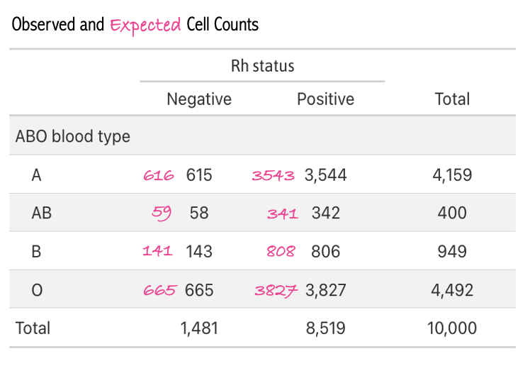
A comparison of the observed cells and our calculated expected cells demonstrates a very close match. Indeed, for each blood type, about 85% of cases are Rh+. This provides evidence that, as expected, ABO type and Rh status are independent of one another.

Apply the contingency table to find corresponding probabilities

Given the contingency table, we can calculate the probabilities for various conditions related to the elements of probability that we’ve studied so far in this Module.

1. What is the probability of Type AB blood?

To find the probability of having Type AB blood, we divide the number of individuals with Type AB blood by the total number of individuals.

\[ P(\text{Type AB}) = \frac{\text{Total with Type AB}}{\text{Total observations}} = \frac{400}{10,000} = 0.0400 \]

This calculation shows that the probability that an individual has Type AB blood is 0.04, by multiplying this probability by 100, we can state that about 4% of the population has Type AB blood.

2. What is the probability of Rh-Negative blood?

The probability of being Rh-Negative is calculated by dividing the total number of individuals with Rh-Negative blood by the total number of individuals.

\[ P(\text{Rh-}) = \frac{\text{Total Rh-Negative}}{\text{Total observations}} = \frac{1,481}{10,000} = 0.1481 \]

This indicates that ~15% of the population is Rh-Negative.

3. What is the probability of having Type O blood or being Rh-Positive?

This question involves the union of two events, that is, the probability that a person either has Type O blood, or is Rh-Positive. To calculate \(P(\text{Type O} \cup \text{Rh+})\) with the contingency table you add up the total number of cases of Type O blood and the total number of cases with Rh-Positive blood, and then from this sum subtract the number of cases with both Type O blood and Rh-Positive blood (i.e., O-) to avoid double counting. This quantity is then divided by the total number of cases (10,000).

In terms of counts from the cross table:

• total Type O cases = 4492

• total Rh-Positive cases = 8519

• both Type O and Rh-Positive cases = 3827

Thus, the probability of Type O or Rh-Positive is calculated as follows:

\[ P(\text{Type O or Rh+}) = \frac{(4,492 + 8,519) - 3,827}{10,000} = 0.9184 \]

4. What is the probability of having Type A blood and Rh-Negative blood?

This question involves the intersection of two events — or the joint probability. It can be written as: \(P(\text{Type A} \cap \text{Rh-})\). Answering this question with the contingency table is quite easy — we just need to find the cell that provides this joint count (N = 615), and divide by the total people observed:

\[ \small P(\text{Type A and Rh-}) = \frac{\text{Total with Type A and Rh-Negative}}{\text{Total observations}} = \frac{615}{10,000} = 0.0615 \]

Therefore, the probability of having Type A blood and being Rh-Negative, assuming independence, is 0.0615 — or expressed as a percentage — ~6% of the sample has Type A blood and is Rh-Negative.

Example 2: ABO status and COVID-19 (dependent events)

In this example, we explore the concept of dependent events in probability using the context of blood types and the risk of contracting COVID-19. Unlike the independent events of ABO and Rh blood status, here we consider the dependency between having Type A blood and the likelihood of contracting COVID-19. We simplify the blood types into two categories: Type A and not Type A (which includes Types B, AB, and O).

Let’s consider simulated data for 10,000 people based on the following parameters:

• Probability of having Type A blood, \(P(\text{Type A})\) = 0.42.

• Average population risk of contracting COVID-19 in a certain situation, \(P(\text{COVID-19})\) = 0.05.

• Individuals with Type A blood have a 1.2 times higher relative risk of contracting COVID-19 compared to the average population risk.

The simulated data are presented in the table below¹.

set.seed(445566)

# Parameters
N <- 10000  # sample size
P_A <- 0.42  # Probability of having Type A blood
P_B <- 0.05  # Base probability of contracting COVID-19
relative_risk_A <- 1.2

# Adjusted probability of contracting COVID-19 for Type A
P_B_given_A <- P_B * relative_risk_A

# Simulate blood type using sample()
blood_type <- sample(c("Type A", "Not Type A"), size = N, replace = TRUE, prob = c(P_A, 1 - P_A))

# Adjust COVID probability for Not Type A to maintain overall P(B)
P_B_given_not_A <- (P_B - P_B_given_A * P_A) / (1 - P_A)

# Generate one set of random numbers for COVID assignment
rand_nums <- runif(N)

# Assign COVID status 
covid_status <- case_when(
  blood_type == "Type A" & rand_nums < P_B_given_A  ~ "Yes",
  blood_type == "Type A" & rand_nums >= P_B_given_A ~ "No",
  blood_type == "Not Type A" & rand_nums < P_B_given_not_A  ~ "Yes",
  TRUE ~ "No"
)

# Create final data frame
a_covid <- tibble(blood_type, covid_status) |> 
  labelled::set_variable_labels(
    blood_type = "Blood Type",
    covid_status = "Individual has COVID-19?"
  )

a_covid |> 
  select(blood_type, covid_status) |> 
  tbl_cross(row = blood_type, col = covid_status) 

	Individual has COVID-19?		Total
	No	Yes
Blood Type
Not Type A	5,528	260	5,788
Type A	3,948	264	4,212
Total	9,476	524	10,000

Apply the contingency table to find corresponding probabilities

Given the contingency table, we can calculate the probabilities for various conditions related to the elements of probability that we’ve studied so far in this Module.

1. What is the probability of Type A blood?

To find the probability of having Type A blood, we divide the number of individuals with Type A blood by the total number of individuals.

\[ P(\text{Type A}) = \frac{\text{Total with Type A}}{\text{Total observations}} = \frac{4212}{10,000} = 0.4212 \]

This calculation shows that there’s about a 42% chance of an individual having Type A blood.

2. What is the probability of contracting COVID-19 among people with Type A blood?

To find the probability of contracting COVID-19 among people with Type A blood, we use the conditional probability formula:

From the provided contingency table, we have:

• Number of Type A individuals with COVID-19 = 264

• Total number of Type A individuals = 4,212

Let’s calculate the probability:

\[ \small P(\text{COVID-19} | \text{Type A}) = \frac{\text{Number of Type A individuals with COVID-19}}{\text{Total number of Type A individuals}} = \frac{264}{4212} = 0.063 \]

The probability of contracting COVID-19 among people with Type A blood, based on the simulated data, is approximately 0.063. This calculation indicates that out of all individuals with Type A blood in the simulated population, about 6.3% are expected to contract COVID-19.

3. What is the probability of contracting COVID-19 among people without Type A blood?

To find the probability of contracting COVID-19 among people with a blood type other than Type A, we use the conditional probability formula:

From the provided contingency table, we have:

• Number of Type B/AB/O individuals with COVID-19 = 260

• Total number of Type B/AB/O individuals = 5,788

Let’s calculate the probability:

\[ \small P(\text{COVID-19} | \text{not Type A}) = \frac{\text{Number of not Type A individuals with COVID-19}}{\text{Total number of not Type A individuals}} = \frac{260}{5788} = 0.045 \]

The chances of contracting COVID-19 among people with Type B, AB or O blood, based on the simulated data, is approximately 4.5%. This calculation indicates that out of all individuals with a blood type other than Type A blood (i.e., Type O, B, or AB) in the simulated population, about 4.5% are expected to contract COVID-19.

Notice that the probability of contracting COVID-19 for people with Type A blood and for people with all other blood types is different — people with Type A blood are more likely to contract COVID-19. This demonstrates the dependence of these two events.

4. What is the probability of having Type A blood or contracting COVID?

To find the probability that a randomly selected person either has Type A blood or contracts COVID-19, we use the formula for the union of two events, denoted as \(P(\text{Type A} \cup \text{COVID-19})\). This represents the probability that a person either has Type A blood, contracts COVID-19, or experiences both.

Given from the contingency table and initial parameters:

• 4212 individuals have Type A blood.
• 524 individuals contracted COVID-19.
• 264 individuals have Type A blood and contracted COVID-19.

\[ P(\text{Type A} \cup \text{COVID}) = \frac{(4,212 + 524) - 264}{10,000} = 0.4472 \]

The probability of either having Type A blood or contracting COVID-19, denoted as \(P(\text{Type A} \cup \text{COVID-19})\), is calculated by adding the number of people in each individual event and then subtracting the number of people who experienced both events, as they are not mutually exclusive. Subtracting the overlap is necessary to avoid double counting those who fall into both categories. The resulting calculation shows that approximately 45% of the population either have Type A blood or have contracted COVID-19.

A Final Example

Let’s explore a final practical example. Imagine that you work for a large corporation, and you were notified that there was an outbreak of COVID-19 at your workplace. Now, you seek to determine if you have the virus too. You have a vacation planned in 3 days — and you are very hopeful that you do not have the virus. You take a rapid antigen test. Based on this scenario, imagine two events:

• Event Test+: Testing positive for COVID-19
• Event COVID+: Actually having COVID-19

Consider the contingency table below that summarizes the relationship between these two events across 1,000 people in your workplace.

• The columns of the table categorize individuals based on their actual COVID-19 status:

  • “No” signifies the individual doesn’t have COVID-19

  • “Yes” signifies the individual has COVID-19

• The rows of the table categorize individuals based on their COVID-19 test results:

  • “Negative” signifies the individual tested negative for COVID-19

  • “Positive” signifies they tested positive for COVID-19

We’ll use this information to consider your scenario as stated above.

test_results |> 
  labelled::set_variable_labels(test_result = "Result of test",
                                has_covid = "Individual has COVID-19?") |> 
  select(test_result, has_covid) |> 
  tbl_cross(row = test_result, col = has_covid) 

	Individual has COVID-19?		Total
	No	Yes
Result of test
Negative	721	19	740
Positive	76	184	260
Total	797	203	1,000

Defining correct and incorrect test results

From this contingency table, we can categorize the cells as follows:

• True Positive (TP): Individuals who actually have COVID-19 and the test correctly identifies them as positive. From the table, there are 184 true positives.
• True Negative (TN): Individuals who do not have COVID-19 and the test correctly identifies them as negative. The table shows 721 true negatives.
• False Positive (FP): Individuals who do not have COVID-19, but the test incorrectly identifies them as positive. According to the table, there are 76 false positives.
• False Negative (FN): Individuals who have COVID-19, but the test incorrectly identifies them as negative. We see 19 false negatives in the table.

As such, two of the cells represent “correct” results of the test (TP and TN cells), but two of the cells represent “incorrect” results of the test (FP and FN).

Based on the cross table we can compute two quantities from the table margins:

• The probability of getting a positive test result: \(P(Test+) = 260/1000 = 0.260\).

• The probability of having COVID-19: \(P(COVID+) = 203/1000 = 0.203\).

Sensitivity

The primary purpose of a screening test, including a COVID-19 rapid antigen test, is to detect the presence of the virus. This is commonly referred to as the test’s sensitivity — that is, its ability to correctly identify those with the disease — and answers the question:

“What is the probability of testing positive for COVID-19 given that I actually have the virus?”

This is mathematically represented as a conditional probability, specifically \(P(Test+|COVID+)\), and can be calculated using the contingency table as follows:

\[\text{Sensitivity} = \frac{TP}{TP + FN}\]

Using the provided data:

\[\text{Sensitivity} = \frac{184}{184 + 19} = 0.906\]

This indicates that the test correctly identifies 91% of individuals who actually have COVID-19. Sensitivity is a critical metric for test manufacturers because it reflects the test’s accuracy in identifying positive cases of the disease.

Specificity

While sensitivity measures a test’s ability to correctly identify those with the disease, specificity is another critical metric in evaluating a screening test. Specificity measures a test’s ability to correctly identify those without the disease, essentially answering the question:

“What is the probability of testing negative for COVID-19 given that I actually do not have the virus?”

This metric is crucial for ensuring that individuals without the disease are not incorrectly identified as having it, which can lead to unnecessary anxiety, further testing, and potentially unwarranted treatment. Given these categories, specificity is mathematically represented as the conditional probability of testing negative given no presence of the disease. In probability theory, conditional probabilities can also be expressed for complementary events. If \(P(Test+|COVID+)\) denotes the probability of a positive test occurring given that the a COVID-19 infection (i.e., the sensitivity of the test in our example), then expressing the probability of the complement of a positive test given the complement of a COVID-19 infection would typically be denoted as \(P(\text{Test+}^c \mid \text{COVID+}^c)\), where the c superscript denotes the complement of the defined event – that is, it represents the probability of testing negative given that one is truly free of the disease.

The specificity measures the proportion of true negatives out of all those who do not have the disease. It’s defined as:

\[ \text{Specificity} = \frac{TN}{TN + FP} \]

Plugging in the numbers:

\[ \text{Specificity} = \frac{721}{721 + 76} = 0.905 \]

This calculation yields the specificity of the test, indicating the probability that the test gives a negative result given that the individual does not have COVID-19.

Specificity, along with sensitivity, provides important information about a test’s accuracy. While sensitivity focuses on correctly identifying disease cases, specificity is concerned with the accurate identification of those without the disease, making both metrics fundamental to understanding and evaluating the performance of diagnostic tests.

Positive Predictive Value (PPV)

While both sensitivity and specificity are important, we might argue that neither of these specifically answer the question that you likely have after testing positive for COVID-19. In this scenario — you most likely are wondering:

“Given that I’ve tested positive for COVID-19, what is the probability that I actually have the virus?”

This question seeks to understand the likelihood of having the disease given a positive test result — mathematically, this is represented as \(P(COVID+|Test+)\), the probability of having COVID-19 given that the test result is positive.

In this example, it’s crucial to recognize that the \(P(Test+|COVID+)\) (the sensitivity of the test) is not inherently equal to \(P(COVID+|Test+)\). This latter probability is called the positive predictive value (PPV), and it measures the probability that individuals who test positive for COVID-19 actually have the virus. It’s defined mathematically as:

\[ PPV = \frac{TP}{TP + FP} \]

Using the provided data:

\[ PPV = \frac{184}{184 + 76} = 0.708 \]

If you tested positive for COVID-19, then the probability that you actually have COVID-19 is 0.71. Despite the high accuracy of the test, nearly 1/3 of people who test positive won’t actually have the virus — this is sometimes referred to as the False Positive Paradox. Even a highly accurate test can yield a surprisingly large number of false positives, particularly when the disease is rare.

Bayes’ Theorem

By defining the positive predictive value (PPV) as the probability that a person has the disease given a positive test result, we apply the principles of Bayes’ theorem. Bayes’ theorem is a foundational concept in probability theory that allows us to update the probability of a condition or hypothesis in light of new evidence. In the case of our example, the positive test result is the new evidence, and the hypothesis being updated is whether you have COVID-19.

Bayes’ theorem is written as:

\[ P(B|A) = \frac{P(A|B) \times P(B)}{P(A)} \]

Notice that we need three pieces of information to solve for \(P(B|A)\) here — which we defined earlier as the positive predictive value (PPV) of the test:

1. \(P(A|B)\), which, in the context of our example is the sensitivity of the COVID-19 rapid antigen test.
2. \(P(B)\), which is the probability of having COVID-19.
3. \(P(A)\), which is the probability of testing positive for COVID-19.

The power of Bayes’ theorem lies in its ability to incorporate prior knowledge about the prevalence of the disease, \(P(B)\), and specific test information, \(P(A∣B)\) and \(P(A)\), to yield a practical and highly relevant probability \(P(B∣A)\) — the PPV. This means that if we know the sensitivity of a test, the prevalence of the disease, and the overall rate of positive tests, we can accurately determine the likelihood that a positive test result truly indicates the presence of the disease, even if we don’t have raw data like we did in our example.

We can plug the corresponding numbers for our example into the formula for Bayes’ Theorem as follows:

\[ P(B|A) = \frac{P(A|B) \times P(B)}{P(A)} = \frac{0.906 \times 0.203}{0.260} = 0.71 \] Notice that this is the PPV solved earlier.

Key takeaway

Understanding the distinction between two conditional probabilities is essential when interpreting test results:

• The Positive Predictive Value (\(P(B|A)\)): \(P(\text{COVID+} | \text{Test+}) = 0.708\)

• The Test Sensitivity (\(P(A|B)\)): \(P(\text{Test+} | \text{COVID+}) = 0.906\)

While sensitivity is a valuable measure of a test’s ability to detect disease when it’s present (and is commonly reported by test manufacturers), it does not tell us how likely a positive test result actually indicates disease. That’s where PPV becomes critical.

PPV answers the question most people care about after testing positive:

“What is the chance I actually have the disease?”

Unlike sensitivity, PPV takes into account not only the test’s accuracy, but also the prevalence of the disease in the population. When a disease is rare, even a highly sensitive and specific test can produce a large number of false positives, leading to a lower PPV.

To solidify these ideas, please watch the following Crash Course Statistics video on Bayesian updating.

Learning Check

After completing this Module, you should be able to answer the following questions:

1. What does a probability of 0.85 mean in everyday language?
2. What is the key distinction between theoretical and empirical probability?
3. How does a data generating process (DGP) help explain observed outcomes?
4. What is the difference between probability and statistics, and how do they relate to one another?
5. How do you use the addition rule to find the probability of Y or Z? What’s different when the events are not mutually exclusive?
6. How do you use the multiplication rule to find the probability of Y and Z? How does this change if Y and Z are dependent?
7. How can you calculate joint and conditional probabilities using a contingency table?
8. What is the positive predictive value (PPV) of a diagnostic test, and how is it different from sensitivity?
9. How do you apply Bayes’ Theorem to estimate the probability that someone has a condition given a positive test result?

Credits

• In writing about the basic rules of probability, I drew from the excellent book entitled Advanced Statistics from an Elementary Point of View as well as The Cartoon Guide to Statistics.
• I was inspired by the Quantitude Podcast Season 3 Episode 16 to create the Bayes’ Theorem example of testing positive for COVID-19 and actually having COVID-19.

Footnotes

1. The simulation of these data is a little more involved and require some code that you haven’t yet learned about — so for now, you can study the code if you like, or just ignore and look at the output.