library(marginaleffects)
library(gtsummary)
library(here)
library(broom)
library(tidyverse)Moderator Models
Module 14
Learning Objectives
By the end of this Module, you should be able to:
- Define moderation in the context of multiple linear regression models
- Identify research questions where the effect of one variable depends on the level of another
- Fit moderation models using multiple linear regression in R
- Interpret model components in moderation models, including main effects and interaction terms
- Explain the difference between parallel slopes models and interaction models
- Visualize moderation by plotting interaction effects and interpreting non-parallel slopes
- Communicate findings from a moderation analysis clearly and effectively, both numerically and visually
Overview
In the regression models we’ve built so far, we’ve assumed that the effect of each predictor on the outcome is additive and constant. That is, we’ve treated predictors as if they each contribute their own fixed part to the outcome, regardless of what the other variables in the model are doing.
But in the real world — especially in psychology and behavioral science — things are rarely that straightforward.
Often, the effect of one variable depends on something else. A therapy might help most people, but not everyone. The impact of stress on mental health might be stronger for people with low social support than for those who feel well-supported. In cases like these, we’re dealing with moderation.
Moderation happens when the magnitude — or even the direction — of a relationship between two variables changes depending on a third variable, known as the moderator.
Understanding moderation helps us move beyond the question, “Does this variable have an effect?” and ask something more insightful:
“When, and for whom, does this variable have an effect?”
This is a powerful shift. In behavioral science, moderation analysis helps us tailor interventions, test more nuanced theories, and uncover meaningful differences across people, situations, or contexts.
In this Module, you’ll learn how to identify and test moderation in your data using regression models. We’ll learn how to fit these models in R, interpret the results, and visualize the effects in ways that make the findings clear and actionable.
Introduction to the Data
We’ll use data from a study published by Allen et al. (2023) in the Journal of Applied Psychology. The researchers pulled data from the Midlife in the United States Study (i.e. the MIDUS Study) — a long-running, nationally representative study of adults in the U.S. funded by the National Institutes of Health. MIDUS is a treasure trove for behavioral science research, offering rich data on health, personality, work, and social relationships across the adult lifespan. And, the data are publically available.
Allen and colleagues examined the causes of work–family conflict (WFC), focusing specifically on adult twin pairs who were balancing both work and family responsibilities. Their goal was to understand whether genetic factors — rather than just situational factors like job or family demands — play a role in shaping how people experience work interfering with family (WIF) and family interfering with work (FIW).
Using data from both monozygotic (MZ) and dizygotic (DZ) twins, the researchers aimed to estimate the extent to which WFC is influenced by heritable traits versus environmental factors.
Why twins? Because comparing MZ and DZ twins allows researchers to explore the role of genetics versus environment. MZ twins share nearly 100% of their genes, while DZ twins, like regular siblings, share about 50%. If MZ twins are more similar to each other on a given trait than DZ twins are, that suggests genetic factors may be at play. But because both types of twins typically grow up in the same family environment, researchers can use this comparison to separate the influence of shared genes from shared environments.
Allen and colleagues found that genetics explained a significant portion of individual differences in both WIF and FIW — especially WIF. They also tested whether the relationships between role demands and WFC were due to causal effects of the environment (like stressful work conditions) or to underlying genetic predispositions. Their findings suggest that work demands affect WIF through situational processes, while family demands are more genetically confounded when predicting FIW.
While we’re not going to replicate the findings from the Allen et al. study, we are using the same dataset to explore a related question about how similar twins are in their experiences of WIF, and whether that similarity depends on zygosity.
We’re going to zoom in on one specific outcome: Work Interference with Family (WIF) — a measure of how much someone’s job interferes with their home life. Our research question is this:
How similar are siblings in a twin pair when it comes to their experiences of WIF? And does that similarity depend on whether they’re MZ or DZ twins?
In other words, we’re asking whether zygosity moderates the concordance in WIF — an ideal setup for learning about moderation analysis.
Let’s load the necessary packages for this Module.
And, import the data frame, called midus_twins_workfamily.Rds.
orig_data <- read_rds(here("data", "midus_twins_workfamily.Rds"))
orig_data |> head(n = 24)
Here’s a listing of all the variables in the data frame (though we’ll only use a subset of these here):
| Variable | Description |
|---|---|
| id | Individual ID |
| fam_id | Family ID |
| time | Study wave: w1, w2, w3 for waves 1 through 3 |
| zyg | Zygosity of twin pair: dz - same sex = dizygotic (male-male or female-female); dz - different sex = dizygotic (male-female); mz = monozygotic |
| wif | Work Interference with Family (wif): Measures how often job demands affect home life in the past year. Responses range from all the time (1) to never (5). Higher scores indicate greater conflict. |
| fiw | Family Interference with Work (fiw): Assesses how often family responsibilities impact work in the past year. Responses range from all the time (1) to never (5). Higher scores indicate greater conflict. |
| jd | Job Demands: Evaluates the intensity of job requirements, including too many demands, insufficient time, and frequent interruptions. Responses range from all the time (1) to never (5), Higher scores indicate greater job demands. |
| fd | Family Demands: Looks at the pressure from family obligations, including excessive demands and frequent interruptions. Responses range from all the time (1) to never (5). Higher scores indicate greater family demands. |
| ext | Extraversion: Personality trait indicating sociability. Responses range from not at all (1) to a lot (4). Higher scores reflect greater extraversion. |
| agr | Agreeableness: Trait showing propensity for kindness and cooperation. Responses range from not at all (1) to a lot (4). Higher scores reflect greater agreeableness. |
| neu | Neuroticism: Personality trait indicating emotional instability. Responses range from not at all (1) to a lot (4). Higher scores reflect greater neuroticism. |
| opn | Openness: Trait related to creativity and willingness to experience new things. Responses range from not at all (1) to a lot (4). Higher scores reflect greater openness. |
| con | Conscientiousness: Trait indicating reliability and diligence. Responses range from not at all (1) to a lot (4). Higher scores reflect greater conscientiousness. |
| lifesat | Life Satisfaction. Responses include 1 = not at all, 2 = a little, 3 = somewhat, 4 = a lot. |
| mh | Mental Health Rating. Responses include 1 = poor, 2 = fair, 3 = good, 4 = very good, 5 = excellent. |
| ph | Physical Health Rating. Responses include 1 = poor, 2 = fair, 3 = good, 4 = very good, 5 = excellent. |
| comph | Comparison of Overall Health to Others Your Age. Responses include 1 = much worse, 2 = somewhat worse, 3 = about the same, 4 = somewhat better, 5 = much better. |
| sex | Sex of twin: 1 = male, 2 = female |
| age | Age of twins in years |
Before we dive into modeling, we need to prepare our data. Here’s what we’re going to do — and why:
Filter to Wave 1 responses: We’ll focus on data from the first wave of MIDUS to keep things simple and consistent.
Keep only monozygotic and same-sex dizygotic twins: We want to reduce variability that might be due to sex differences, so we’ll focus only on twin pairs who are both male or both female. That includes all MZ twins (who are always same-sex) and same-sex DZ twins.
Assign a “twin 1” and “twin 2” label within each pair: The original data has one row per person. To compare twins within pairs, we need to create one row per pair, with variables for each twin. To do that, we label each individual as “twin 1” or “twin 2.”
Reshape from long to wide format: We restructure the data so that each row represents a full twin pair. That way, we can directly compare values like wif_twin1 and wif_twin2.
Add a variable to describe the sex composition of each pair: This isn’t necessary for the main analysis, but it can help later if we want to explore differences by sex (e.g., male vs. female twins).
Select only the variables we’ll use: To stay focused, we’ll keep just the core variables for this activity: family ID, zygosity, age, sex pair type, and each twin’s WIF score.
Drop incomplete twin pairs: We remove any pairs that are missing data on the key variables to ensure a clean analysis for the purpose of instruction.
df <-
  orig_data |>
  filter(time == "w1") |>
  filter(zyg %in% c("mz", "dz - same sex")) |>
  group_by(fam_id) |>
  mutate(twin_identifier = case_when(row_number() == 1 ~ "_twin1",
                                     row_number() == 2 ~ "_twin2")) |>
  ungroup() |>
  pivot_wider(
    id_cols = c(fam_id, zyg, time, age),
    names_from = twin_identifier,
    names_sep = "",
    values_from = c(sex, wif, fiw, jd, fd, agr, opn, con, ext, neu, lifesat, mh, ph, comph),
  ) |>
  mutate(sex_pair = case_when(sex_twin1 == 1 & sex_twin2 == 1 ~ "male twins",
                             sex_twin1 == 2 & sex_twin2 == 2 ~ "female twins",
                             (sex_twin1 == 1 & sex_twin2 == 2) |
                               (sex_twin1 == 2 & sex_twin2 == 1) ~ "male-female twins")) |>
  select(fam_id, zyg, age, sex_pair, wif_twin1, wif_twin2) |>
  drop_na()

df |> head()
Visualize Concordance of WIF Across Twin Types
Before we build any models, let’s just look at the data.
Specifically, we want to know:
How similar are twins when it comes to work-family conflict?
And does that similarity differ depending on whether they’re MZ or DZ twins?
If two twins in a pair have very similar experiences, we’d expect their scores to be about the same. That means, for any given pair, if Twin 1 reports a high level of WIF, Twin 2 should also report a high level — and if Twin 1 reports a low level, so should Twin 2. In other words, their points should fall close to a straight line on the plot, where Twin 1’s score is roughly equal to Twin 2’s score.
The closer the dots are to this line, the stronger the similarity (or concordance) between twins. If the dots are more scattered — far from the line — it means the twins in a pair are having different experiences, and there’s less similarity in their WIF scores.
This kind of plot gives us an intuitive sense of how closely matched the twins are, which sets the stage for testing whether that similarity differs depending on zygosity (i.e., whether they are MZ or DZ twins).
We’ll start by creating two separate plots — one for MZ twins and one for same-sex DZ twins:
# Set color palette for zygosity
levels <- c("mz", "dz - same sex")
colors <- c("#2F9599", "#A7226E")
my_colors_zyg <- setNames(colors, levels)

df |>
  ggplot(mapping = aes(x = wif_twin1, y = wif_twin2, fill = zyg, color = zyg)) +
  geom_jitter() +
  geom_smooth(method = "lm", formula = y ~ x) +
  scale_color_manual(values = my_colors_zyg) +
  scale_fill_manual(values = my_colors_zyg) +
  facet_wrap(~zyg) +
  theme_minimal() +
  theme(legend.position = "none") +
  labs(title = "Association of WIF between siblings in a twin pair",
       x = "WIF for Twin #2",
       y = "WIF for Twin #1")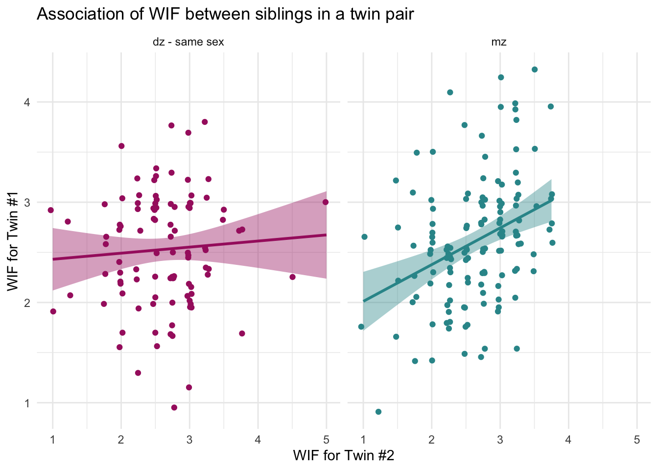
If you’d prefer a single plot that shows both groups together, we can show both lines on the same axes and include a legend as follows:
df |> ggplot(mapping = aes(x = wif_twin1, y = wif_twin2, fill = zyg, color = zyg)) +
  geom_jitter(alpha = 0.75) +
  geom_smooth(method = "lm", formula = y ~ x) +
  theme_minimal() +
  scale_color_manual(values = my_colors_zyg) +
  scale_fill_manual(values = my_colors_zyg) +
  labs(title = "Association of WIF between siblings in a twin pair",
       x = "WIF for Twin #2",
       y = "WIF for Twin #1",
       fill = "Zygosity",
       color = "Zygosity")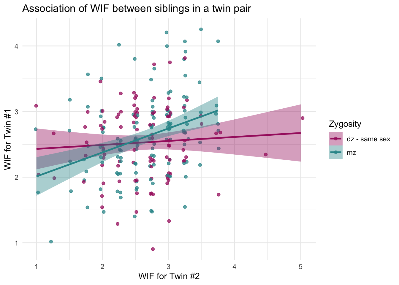
What do these graphs show?
For dizygotic (DZ) twins, the points are more scattered and the line is relatively flat. That suggests a weak relationship — if one twin reports high work-family conflict, the other twin might not. Their experiences are only loosely connected.
For monozygotic (MZ) twins, the line is steeper and the data points are more tightly clustered about the best fit line. This indicates a stronger relationship — when one MZ twin reports high conflict, the other usually does too. Their experiences are more aligned.
Why does this matter?
This visual gives us our first hint that zygosity might influence how similar twins are in their experiences of work interfering with family life.
In other words, the relationship between one twin’s WIF score and the other’s doesn’t appear to be the same for all twin pairs — it seems to differ depending on zygosity. For MZ twins, the association looks stronger (a steeper slope, with the points more tightly clustered about the best fit line); for DZ twins, it looks weaker (a flatter slope).
And that’s the big idea behind moderation:
Does the effect of one variable on another depend on something else?
In this case, we’re asking whether the effect of Twin 2’s WIF score on Twin 1’s WIF score depends on whether the twins are identical or fraternal.
Now that we’ve spotted a possible moderation pattern in the graph, we’re ready to test it more formally using regression.
Fit Separate Regression Models for MZ and DZ Twins
Let’s take the next step: use regression to model the similarity in WIF between twins.
We’re going to fit two separate simple linear regression (SLR) models — one for MZ twins and one for same-sex DZ twins. In both models, we’ll predict Twin 1’s WIF score using Twin 2’s WIF score.
Why build two models? Because we want to know whether the nature of the relationship is different for MZ and DZ twins — and this approach allows us to estimate those relationships separately.
But before we do that, we need to make one small adjustment.
Center the key predictor
One of our predictors is wif_twin2, which ranges from 1 to 5. But notice that a value of 0 doesn’t naturally occur — and that makes interpreting the intercept in our models harder.
To make the intercept more meaningful, we’ll center the variable by subtracting 1 from each value. That way, a value of 0 on the new variable (wif_twin2.c) corresponds to the lowest possible WIF score (1 on the original scale). This makes the intercept easier to interpret: it represents the predicted score for Twin 1 when Twin 2 reports the lowest possible WIF.
We’ll also split the data into two separate groups: mz for MZ twins and dz for same-sex DZ twins.
df <-
  df |>
  mutate(zyg = factor(zyg),
         zyg = relevel(zyg, ref = "mz")) |>
  mutate(wif_twin2.c = wif_twin2 - 1)

# create subsetted dataframes
dz <- df |> filter(zyg == "dz - same sex")
mz <- df |> filter(zyg == "mz")
Fit the models
Now we’ll fit two simple linear regression models (and additionally estimate the correlation):
Model for DZ twins
 # Fit the regression model and display tidy results
model_dz <- lm(wif_twin1 ~ wif_twin2.c, data = dz)

model_dz |>
  tidy(conf.int = TRUE, conf.level = 0.95) |>
  select(term, estimate, std.error, conf.low, conf.high)
# Compute the correlation
dz |>
select(wif_twin1, wif_twin2) |>
corrr::correlate()Correlation computed with
• Method: 'pearson'
• Missing treated using: 'pairwise.complete.obs'Model for MZ twins
# Fit the regression model and display tidy results
model_mz <- lm(wif_twin1 ~ wif_twin2.c, data = mz)

model_mz |>
  tidy(conf.int = TRUE, conf.level = 0.95) |>
  select(term, estimate, std.error, conf.low, conf.high)
# Compute the correlation
mz |>
select(wif_twin1, wif_twin2) |>
corrr::correlate()Correlation computed with
• Method: 'pearson'
• Missing treated using: 'pairwise.complete.obs'Interpret the results
Each SLR model has:
An intercept, which tells us the predicted WIF for Twin 1 when Twin 2 reports the lowest possible WIF (remember, that’s a 1 on the original scale).
A slope, which tells us how much Twin 1’s WIF score is expected to change for each one-unit increase in Twin 2’s WIF score.
Let’s break it down:
For MZ twins, the slope is about 0.34 (95% CI: 0.18 to 0.49). That’s a moderate, positive relationship. When one twin reports more work-family conflict, their genetically identical sibling tends to as well. Additionally, the correlation is moderate (\(r\) = 0.35).
For DZ twins, the slope is much smaller — around 0.08 (95% CI: –0.15 to 0.30). The relationship is weaker and the confidence interval includes 0, meaning it’s plausible that there’s no real relationship in the DZ group. Additionally, the correlation is small (\(r\) = 0.07).
Why this matters
This tells us something important:
The concordance in WIF appears to be stronger for MZ twins than for DZ twins.
This is exactly what we expect if genetic similarity moderates how similar twins are in their work-family conflict.
We’ve tested this by fitting the models separately — but next, we’ll combine everything into one model. This will allow us to formally test whether the difference in slopes between MZ and DZ twins is statistically meaningful.
A Combined Model: Parallel Slopes
So far, we’ve looked at two separate regression models — one for MZ twins and one for DZ twins. That approach gave us a clear sense of how WIF scores relate within each group. But now, we want to pull everything together into one model.
Why combine the groups? Because sometimes we want to:
- Compare groups more efficiently.
- Test differences directly within a single model.
- Control for certain variables, while assessing the effect of others.
Let’s start by fitting a model that assumes the relationship between Twin 1’s and Twin 2’s WIF scores is the same across groups, except for a difference in overall level. This is called a parallel slopes model.
lm_ps <-
  lm(wif_twin1 ~ wif_twin2.c + zyg, data = df)

lm_ps |>
  tidy(conf.int = TRUE, conf.level = 0.95) |>
  select(term, estimate, std.error, conf.low, conf.high)
Interpret the model coefficients
Let’s walk through what each part of the model output means:
Intercept (2.26): This is the predicted WIF for Twin 1 when Twin 2’s WIF is 1 (because we centered the predictor at 1) and the twins are monozygotic (the reference group for zyg). That is, when wif_twin2.c == 0 and zyg == 0.
Slope for wif_twin2.c (0.24): This is the effect of Twin 2’s WIF on Twin 1’s WIF, holding constant zygosity. In other words, if we compare two MZ twins or two DZ twins, this coefficient represents the expected change in WIF for Twin 1 for each one-unit increase in WIF for Twin 2.
Slope for zyg (0.01): This is the expected difference in Twin 1’s WIF between DZ twins (when zyg equals 1) and MZ twins (when zyg equals 0), holding constant WIF for Twin 2.
What is a parallel slopes model?
In this model:
- The slope for WIF concordance is the same for both MZ and DZ twins.
- The difference between the groups is in their intercepts, not in their slopes.
That’s why it’s called “parallel slopes” — the two lines (one for each twin type) have the same steepness but start at different places on the y-axis.
Visualize the model
Here’s a plot of the predicted WIF scores for Twin 1, based on Twin 2’s scores and zygosity. The predictions() function from the marginaleffects package is used to compute predicted values — and then we can plot the predictions to show the fitted lines.
pred_data_ps <-
  predictions(
  lm_ps,
  conf_level = 0.95,
  df = insight::get_df(lm_ps),
  newdata = datagrid(
    wif_twin2.c = seq(0, 3, by = 0.05),
    zyg = unique    # one curve per zygosity
  )
) |>
  as_tibble()

pred_data_ps |> select(zyg, estimate, conf.low, conf.high)
pred_data_ps |>
ggplot(mapping = aes(x = wif_twin2.c, y = estimate, color = zyg, fill = zyg)) +
geom_ribbon(aes(ymin = conf.low, ymax = conf.high), alpha = 0.15) +
geom_line() +
scale_color_manual(values = my_colors_zyg, name = "Zygosity") +
scale_fill_manual(values = my_colors_zyg, name = "Zygosity") +
labs(
title = "Fitted concordance in WIF between twin pairs",
subtitle = "Parallel slopes model",
x = "Work interfering with family for twin 2",
y = "Predicted work interfering with family for twin 1"
) +
theme_minimal() +
theme(legend.position = "right")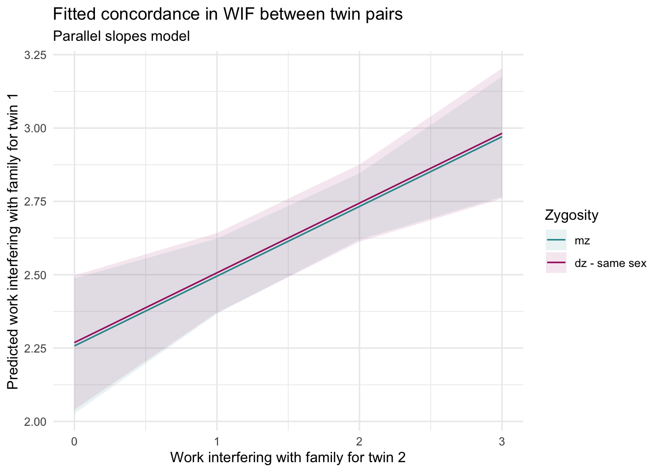
How is this code working
We begin with the predictions() function to generate predicted values from the fitted model lm_ps. The function computes the expected outcome for a grid of input values, here varying Twin 2’s WIF score from 0 to 3 while repeating the calculation for each level of zygosity (e.g., identical vs. fraternal twins). The argument conf_level = 0.95 requests 95% confidence intervals for each prediction and argument df = insight::get_df(lm_ps), tells the function to use the proper degrees of freedom from the fitted model to construct the CI. These results are converted into a tibble for easy plotting, and the zygosity variable is ordered consistently for labeling and color mapping.
How to interpret this plot
Each line shows the predicted WIF for Twin 1 as Twin 2’s WIF increases, separately for MZ and DZ twins.
The slopes are the same — they rise at the same rate.
The lines are vertically offset — DZ twins tend to have very slightly higher WIF for Twin 1 than MZ twins.
This model assumes that the concordance is equally strong in both groups, but that the average level of WIF might differ by zygosity.
Compute slopes by zygosity
Let’s confirm the parallel slopes with the slopes() function from the marginaleffects package to see whether the estimated slopes are truly the same across groups.
lm_ps |>
  slopes(variables = "wif_twin2.c", by = "zyg") |>
  as_tibble() |>
  select(term, zyg, estimate)
Here’s what’s happening in this code chunk:
Model Input (
lm_ps): This is the regression model we previously fit, and we pipe it into the slopes() function.slopes(variables = "wif_twin2.c", by = "zyg"): This tells slopes() to calculate the slope of wif_twin2.c separately for each level of the moderator (zyg).- For example, it estimates how strongly Twin 2’s WIF score predicts Twin 1’s WIF score in monozygotic pairs vs. dizygotic pairs.
as_tibble(): This converts the result to a tidy tibble for easier manipulation and viewing with tidyverse tools.
The output confirms what the model assumes: the effect of Twin 2’s WIF on Twin 1’s WIF is the same across twin types.
What’s next?
This model is helpful — but remember what we saw earlier? The relationship looked larger for MZ twins than for DZ twins. So maybe assuming the same slope isn’t quite right.
In the next section, we’ll relax the parallel slopes assumption and fit a model that allows for different slopes — a true moderation model with an interaction term.
Non-Parallel Slopes: Moderation via Interaction
In the previous model, we assumed that the relationship between Twin 1’s and Twin 2’s WIF scores was the same for both MZ and DZ twins — the only difference was in the average starting point (the intercept).
But what if that assumption doesn’t hold?
What if the nature of the relationship itself differs between groups?
This brings us to the idea of moderation: when the effect of one variable depends on the level of another. In our case, we’re asking:
Does zygosity (MZ vs. DZ) change the magnitude of the relationship between Twin 1’s and Twin 2’s WIF scores?
To test this, we’ll fit a model that includes an interaction between Twin 2’s WIF score and zygosity. This model allows for non-parallel slopes — in other words, it allows the effect of Twin 2’s WIF to differ by zygosity.
A general guide to interpreting interactions
Before we fit our model to test for moderation, let’s pause to understand how to interpret regression coefficients when an interaction term is included.
When your model includes an interaction between two variables — for example, \(X\) and \(Z\), it allows the effect of one variable (X) to depend on the level of another variable (Z). In our applied example for this Module:
\(X\) = WIF for Twin 2 (our main predictor)
\(Z\) = Zygosity (our proposed moderator)
To include an interaction term in a regression model in R, use an asterisk (*) between the two variables:
lm(Y ~ X*Z)This expands to include the main effects of both X and Z, as well as their interaction (X:Z). It’s shorthand for:
lm(Y ~ X + Z + X:Z)The resultant fitted model looks like this:
\[ \hat{Y} = b_0+(b_1\times{X})+(b_2\times{Z})+(b_3\times{X}\times{Z}) \]
Each part of this equation plays a specific role:
\(b_0\) (the intercept): This represents the predicted \(Y\) when \(X\) and \(Z\) are both 0.
\(b_1\) (the coefficient for X): This tells us the effect of \(X\) when \(Z = 0\).
\(b_2\) (the coefficient for Z): This tells us the effect of \(Z\) when \(X = 0\).
\(b_3\) (the interaction term): This tells us how the effect of \(X\) changes as \(Z\) changes — specifically, the expected change in the effect of \(X\) for a one-unit increase in \(Z\).
This exposition should make it clear why we need to ensure that a score of 0 is meaningful for both \(X\) and \(Z\). For instance, if \(X\) is measured on a scale from 1 to 5, then interpreting the “effect of \(Z\) when \(X = 0\)” doesn’t make much sense. That’s exactly why we centered WIF for Twin 2 earlier — to give 0 a meaningful interpretation.
To make interaction models interpretable, we often redefine or transform variables so that 0 corresponds to a useful score/value — such as the lowest possible value on a scale, a neutral midpoint, or a reference category (e.g., when \(X\) or \(Z\) are categorial variables). This helps ensure that the model’s coefficients reflect real-world scenarios and tell a clear and meaningful story.
Fit the interaction model
lm_int <-
  lm(wif_twin1 ~ wif_twin2.c*zyg, data = df)

lm_int |>
  tidy(conf.int = TRUE, conf.level = 0.95) |>
  select(term, estimate, std.error, conf.low, conf.high)
Interpret the model coefficients
Let’s walk through what each part of the model output means:
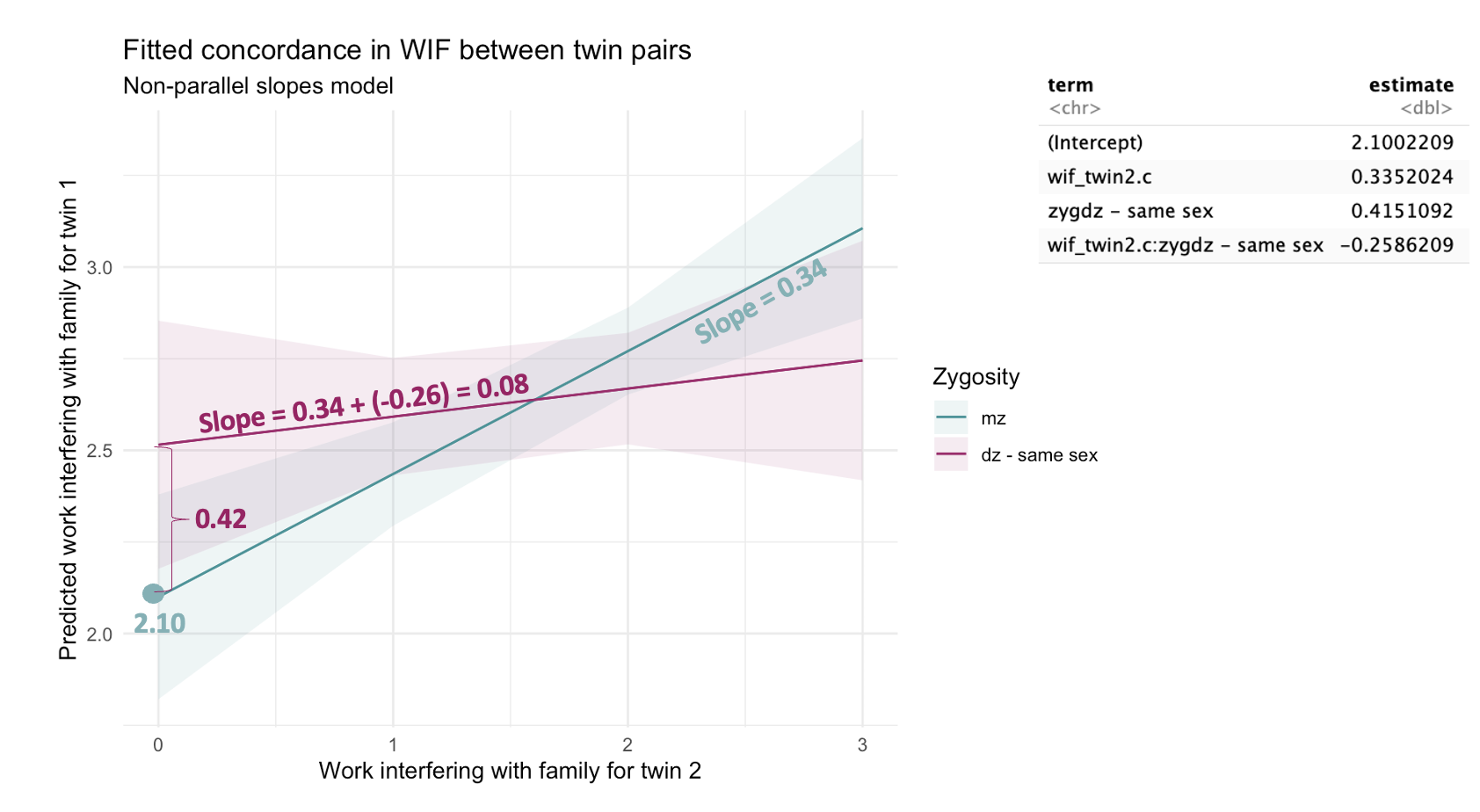
Intercept (2.10): This is the predicted WIF for Twin 1 when Twin 2’s WIF is 1 (because we centered the predictor at 1) and the twins are monozygotic (the reference group).
Slope for wif_twin2.c (0.34): This is the effect of Twin 2’s WIF on Twin 1’s WIF for MZ twins (the reference group).
Slope for zyg (0.42): This tells us that when Twin 2’s WIF is at its lowest (wif_twin2.c equals 0), DZ twins tend to report higher WIF for Twin 1 than MZ twins (but the confidence interval includes zero, so we should interpret with caution).
Slope for interaction term, wif_twin2.c:zyg, (–0.26): This term tells us how the relationship between Twin 2’s WIF and Twin 1’s WIF changes for DZ twins compared to MZ twins. This is the coefficient that speaks to whether there is moderation.
Since MZ twins are the reference group, the slope for DZ twins is computed as:
0.34 + (–0.26) = 0.08(where 0.34 is the slope for MZ twins).That means DZ twins show a weaker concordance — their WIF scores are less strongly related.
The 95% confidence interval for this interaction is [–0.52, 0.006], which includes zero, but just barely. This means we can’t rule out the possibility that there’s no true moderation effect, but there’s also evidence pointing toward a potentially meaningful difference.
Interpreting effects on the “cusp” of significance
In real-world research, we often face this kind of gray area. Rather than making a yes/no decision, this is a good moment to reflect:
- Is the estimated effect practically important?
- Is the uncertainty narrow enough that we can say something useful?
- Should we look for replication or explore the pattern in other datasets?
For now, we can cautiously say that the data hint at a moderation effect, but we’d need more evidence to be confident.
Visualize the interaction
pred_data_int <-
  predictions(
  lm_int,
  conf_level = 0.95,
  df = insight::get_df(lm_int),
  newdata = datagrid(
    wif_twin2.c = seq(0, 3, by = 0.05),
    zyg = unique    # one curve per zygosity
  )
) |>
  as_tibble()

pred_data_int |> select(zyg, estimate, conf.low, conf.high)
pred_data_int |>
ggplot(mapping = aes(x = wif_twin2.c, y = estimate, color = zyg, fill = zyg)) +
geom_ribbon(aes(ymin = conf.low, ymax = conf.high), alpha = 0.15) +
geom_line() +
scale_color_manual(values = my_colors_zyg, name = "Zygosity") +
scale_fill_manual(values = my_colors_zyg, name = "Zygosity") +
labs(
title = "Fitted concordance in WIF between twin pairs",
subtitle = "Non-Parallel slopes model",
x = "Work interfering with family for twin 2",
y = "Predicted work interfering with family for twin 1"
) +
theme_minimal() +
theme(legend.position = "right")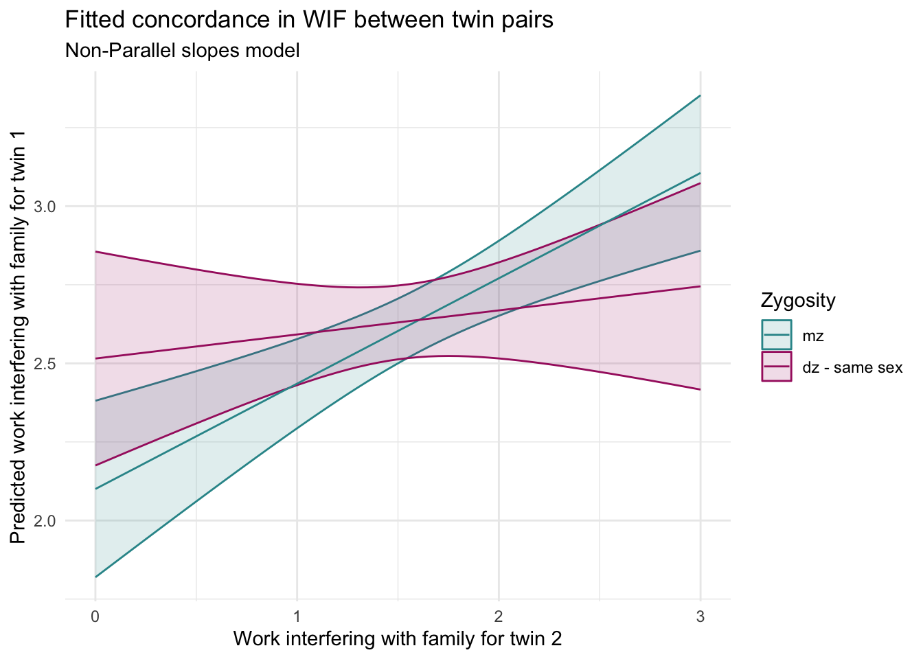
Compute slopes by zygosity
Additionally, we can use the slopes() function again — this time, it will estimate the slope for each group based on the interaction model.
lm_int |>
  slopes(variables = "wif_twin2.c",
         by = "zyg",
         df = insight::get_df(lm_int)) |>
  as_tibble() |>
  select(term, zyg, estimate, std.error, conf.low, conf.high)
Here’s what we see:
MZ twins: slope = 0.34 (95% CI: 0.17 to 0.50) — a clear, moderate positive relationship.
DZ twins: slope = 0.08 (95% CI includes 0) — a weak and uncertain relationship.
Compute the simple slopes manually
While the marginaleffects package job does a fantastic job of automating these outputs, it is instructive to compute the equations that relate WIF for Twin 2 to WIF for Twin 1 by zygosity ourselves. This should help build your intuition for what is happening.
First, recognize that, in terms of the point estimates (listed under estimate in the table produced using tidy()) the interaction model is simply reproducing the same information that we garnered from fitting the two models separately at the start of our exploration (in the section entitled “Fit seperate regression models”).
For reference, the equations from those two separate models are as follows, where \({y_i}\) represents the variable wif_twin1 and \({x_i}\) represents the variable wif_twin2.c.
Equation 1 (For dz twins, \({z_i}\) == “dz - same sex”)): \(\hat{y_i} = 2.52+(0.08\times{x_i})\)
Equation 2 (For mz twins, \({z_i}\) == “mz”): \(\hat{y_i} = 2.10+(0.34\times{x_i})\)
Now, let’s match this up to the output from our fitted model in which zygosity moderates the concordance of WIF, which can be written in equation form as follows (where \(x_i\) represents wif_twin2.c, \(z_i\) represents zyg, and \({x_i}\times{z_i}\) represents the interaction between wif_twin2.c and zyg:
\[ \hat{y_i} = 2.10+(0.34\times{x_i})+(0.42\times{z_i})+(-0.26\times{x_i}\times{z_i}) \] To solve the equation for DZ twins we plug in 1 for \(z_i\):
\[ \hat{y_i} = 2.10+(0.34\times{x_i})+(0.42\times1)+(-0.26\times{x_i}\times1) \] \[ \hat{y_i} = 2.52+(0.08\times{x_i}) \] To solve the equation for MZ twins we plug in 0 for \(z_i\):
\[ \hat{y_i} = 2.10+(0.34\times{x_i})+(0.42\times0)+(-0.26\times{x_i}\times0) \] \[ \hat{y_i} = 2.10+(0.34\times{x_i}) \]
What this tells us?
The plot and the output together suggest that:
MZ twins are more similar in their experiences of work-family conflict.
DZ twins are less similar, and the concordance may even be negligible.
This provides some preliminary evidence that zygosity moderates concordance of WIF between twin pairs.
In other words, the effect of Twin 2’s WIF score may depend on whether the twins are MZ or DZ, but given that the 95% CI for the interaction term includes 0, we need to seek further evidence.
The annotated figure below maps all of this information onto our non-parallel slopes graph.
Learning Check
After completing this Module, you should be able to answer the following questions:
- What is moderation, and how does it differ from a simple additive relationship in regression?
- How can you identify whether a moderation effect might be present by visualizing the data?
- What does an interaction term in a regression model represent conceptually and statistically?
- Why is it helpful to center variables before including them in an interaction model?
- What is the difference between a parallel slopes model and a moderation model?
- How do you interpret the slope of a predictor when it is part of an interaction term?
- How do you use the plot_predictions() function to visualize interaction effects?
- What does it mean if the 95% CI for the interaction term includes 0?
- How can you use the slopes() function to estimate simple slopes for each group?
- How does including an interaction term allow us to ask and answer more nuanced research questions in behavioral science?