Simple Linear Regression
Module 10

Learning Objectives
By the end of this Module, you should be able to:
- Explain the purpose and usefulness of simple linear regression (SLR) in modeling relationships between two continuous variables
- Describe the components of the SLR equation, including the intercept and slope
- Interpret the meaning of the intercept and slope in applied contexts
- Define and calculate a predicted value (\(\hat{y}\)) and a residual (\(e_i\))
- Visualize and evaluate the appropriateness of fitting a straight line to a scatterplot
- Understand the least squares criterion and how it determines the best-fitting line
- Implement a simple linear regression model in R using lm()
- Extract and interpret model outputs using tidy(), augment(), and glance()
- Interpret the \(R^2\) value as the proportion of variance in the outcome explained by the predictor
- Differentiate between the slope (unstandardized effect) and correlation coefficient (standardized effect)
- Explain how regression equations can be used for prediction and forecasting in applied research
Overview
In the social and behavioral sciences, we’re rarely satisfied with studying just one variable in isolation. Instead, we’re driven by questions about relationships: How does one factor influence or predict another? For example, do people who sleep more tend to report better mood the next day? Are higher levels of perceived stress associated with increased symptoms of anxiety? Can time spent on social media predict self-esteem scores among adolescents?
To explore these kinds of questions, we use statistical models — tools that help us detect meaningful patterns, quantify associations, and make predictions, all while accounting for the inherent variability in human behavior.
In this Module, you’ll learn to use one of the most widely used and conceptually intuitive models: simple linear regression. This technique helps us describe the relationship between two continuous variables by fitting a straight line through the data — a line that summarizes the trend while recognizing that no model is perfect.
With simple linear regression, we can:
Estimate how much change in an outcome (like anxiety symptoms) is associated with a one-unit change in a predictor (like perceived stress)
Predict outcomes for new cases based on what we’ve observed in the data
Assess how well our predictor explains variability in the outcome
By the end of this Module, you’ll know how to construct, interpret, and evaluate a simple linear regression model — and use it as a foundation for asking and answering meaningful questions with your own data.
A prior example revisted
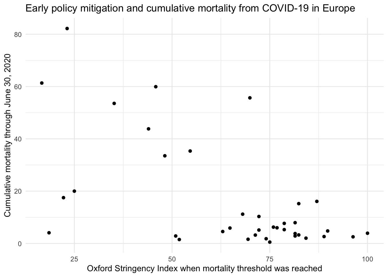
Back in Module 03, we explored data compiled by the Centers for Disease Control and Prevention (CDC) to examine a critical public health question: Did countries that adopted stricter COVID-19 mitigation policies experience fewer deaths? The dataset included information from European countries, capturing two key variables:
Mitigation strictness: Measured using the Oxford Stringency Index — a score that reflects how each country responded to the COVID-19 outbreak in the very early days of the pandemic.
COVID-19 mortality: The total number of deaths attributed to COVID-19 by June 30, 2020.
We visualized these data using a scatterplot to see whether variation in policy strictness was associated with variation in cumulative mortality.
At the time, we noted a general trend: countries with stricter early mitigation efforts tended to report lower death tolls. But our approach was informal — we relied on visual impressions rather than a formal model.
Now that we’re ready to move into simple linear regression, this is the perfect time to revisit that example.
Setting the stage for regression
What if we wanted to go beyond describing the trend and actually quantify the relationship between mitigation policies and mortality? For instance:
How much lower was mortality, on average, for each one-point increase in the stringency index?
Can we predict the expected mortality level for a country with a particular stringency score?
How well does policy stringency explain variation in mortality outcomes across countries?
To answer questions like these, we can fit a simple linear regression model, which allows us to describe the relationship between two continuous variables using a straight line.
Let’s add that line to our scatterplot:
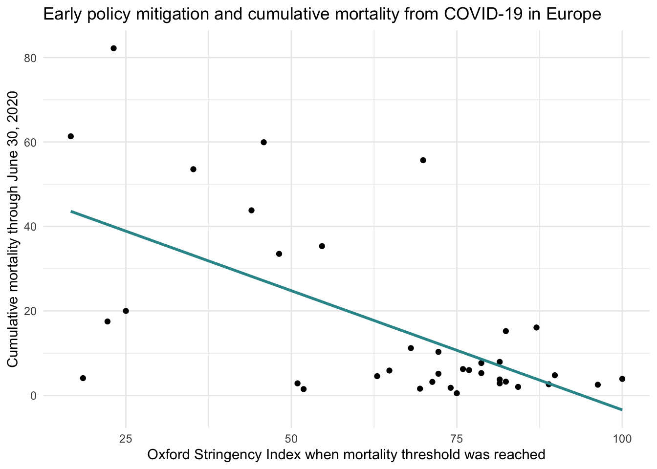
As you can see, the best fit line slopes downward, reflecting a negative relationship: as the stringency of mitigation policies increases, COVID-19 mortality tends to decrease.
From visual insight to statistical model
In this Module, we’ll build on this example to understand how that line is constructed, what its slope and intercept mean, and how well it actually fits the data. You’ll learn how simple linear regression helps us:
Model relationships between continuous variables
Make predictions using an equation
Assess how much of the outcome’s variability is explained by the predictor
By the end of the Module, you’ll be able to formally analyze patterns like the one we saw in this COVID-19 example — using regression as both a descriptive and a predictive tool.
Before we dig into the content, to build your intuition about regression, please watch the following Crash Course Statistics video on Regression. Please note that the video includes an overview of fitting regression models, as well as inference testing (with topics such as degrees of freedom, test statistics, and test distributions). You don’t need to worry about the inference parts for now — we’ll study these topics and techniques later in the course.
Mathematical vs. Statistical Models
Mathematical models
We will use linear models to describe the relationship between two variables. Though you may not have studied or used linear models for prediction before, we often use models to predict outcomes in everyday life. In particular we often use mathematical models to solve problems or make conversions. Mathematical models are deterministic. Once the “rule” is known, the mathematical model can be used to perfectly fit the data. That is, we can perfectly predict the outcome.
Examples of mathematical models include:
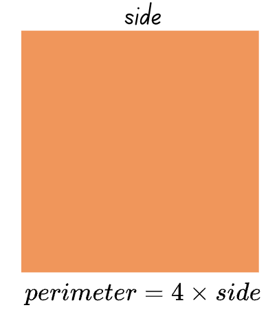
Perimeter of a square \(= 4 \times (length\,of\,side)\)
Area of a square \(= (length\,of\,side)^2\)
Convert Fahrenheit to Celsius: \(C = (F - 32)\cdot\frac{5}{9}\)
Let’s explore the first example. The data frame below represents 25 squares. For each square, the length of a side, and the perimeter are recorded.
Now, let’s use the formula for finding the perimeter based on the length of a side to predict the perimeter for each square. We will use the mutate() function to accomplish this task. Additionally, let’s compute the difference between the observed perimeter and the predicted perimeter based on the formula.
squares <- squares  |>
  mutate(predicted_perimeter = side * 4) |>
  mutate(diff = perimeter - predicted_perimeter)

squares
Not surprisingly, we see that the predicted perimeter that we obtain by applying the formula is precisely the same as the perimeter measurement. This is because this formula is a mathematical model.
Statistical models
While mathematical models are incredibly useful for describing idealized systems, in this course we focus on statistical models, which are better suited to the messy and unpredictable nature of social science data. Unlike mathematical models, statistical models are not deterministic. They recognize that:
We rarely include all the important predictors,
We often measure variables with error, and
People (or schools, organizations, animals—whatever we’re studying) differ in how they behave.
Statistical models allow for uncertainty and individual variability by including a residual term — this captures the part of the outcome that our model doesn’t explain. We can express this idea with a simple equation:
\[\text{Outcome} = \text{Systematic Component} + \text{Residual}\]
This equation helps us break down the total variation in our outcome into two parts:
The systematic component, explained by the predictors we’ve included in our model, and
The residual, which captures the leftover variation due to omitted variables, measurement error, and individual differences.
Let’s return to the COVID-19 mitigation policies example. Suppose we find that countries with stricter policies tend to have fewer deaths — this reflects a clear systematic pattern in the data. However, not every country follows this trend exactly. As you can see in the graph, the data points don’t all fall perfectly on the line relating the predictor to the outcome (i.e., the regression line). If our model were a perfect fit, each point would lie exactly on that line. Instead, some countries have higher or lower mortality than the model predicts. This leftover variation — the residual — captures what the model doesn’t explain. It could reflect differences in healthcare systems, population demographics, reporting practices, or cultural factors not included in the model.
In this Module, we’ll begin learning how to use SLR to model relationships between two continuous variables. SLR allows us to quantify associations, make predictions, and gain insight into how one variable tends to vary as another varies — even when the data are noisy or imperfect.
Introduction to the Data
The substantive focus of this Module is a timely and relevant one: predicting U.S. presidential election outcomes. The individuals elected to public office have far-reaching influence over national policies that shape health, welfare, economic stability, and prosperity for all. Understanding what drives voter behavior is critical for researchers in the social and behavioral sciences.
We will examine a statistical model that has been used to forecast U.S. presidential elections: the Bread and Peace Model, developed by political economist Douglas A. Hibbs. This model is widely recognized for its simplicity and explanatory power.
According to Hibbs, postwar U.S. presidential elections largely function as referenda on the incumbent party’s performance during its term. Specifically, two key variables account for most of the variation in the incumbent party’s share of the two-party vote:
Economic growth: Voters tend to reward the incumbent party when the economy performs well, measured by the weighted-average growth in per capita real disposable personal income.
Military casualties: Voters tend to penalize the incumbent party when there are high cumulative U.S. military fatalities from unprovoked foreign conflicts, scaled by population.
In other words, the likelihood of the incumbent party remaining in power depends on how well the country has fared economically and whether it has experienced costly military engagements.
We’ll start simple. In this Module we will consider a single outcome (election results of US presidential elections) and a single predictor (growth in personal income over the preceding presidential term). To estimate the Bread and Peace model, we will use data compiled by Drew Thomas (2020).
To get started, we need to import the libraries needed for this Module:
library(gtsummary)
library(skimr)
library(here)
library(broom)
library(tidyverse)
In the data frame that we will use, called bread_peace.Rds, each row of data considers a US presidential election. The following variables are included:
| Variable | Description |
|---|---|
| year | Presidential election year |
| vote | Percentage share of the two-party vote received by the incumbent party’s candidate. |
| growth | The quarter-on-quarter percentage rate of growth of per capita real disposable personal income expressed at annual rates |
| fatalities | The cumulative number of American military fatalities per million of the US population |
| wars | A list of the wars of the term if fatalities > 0 |
| inc_party_candidate | The name of the incumbent party candidate |
| other_party_candidate | The name of the other party candidate |
| inc_party | An indicator of the incumbent party (D = Democrat, R = Republican) |
We will estimate how well growth in income of US residents during the preceding presidential term predicts the share of the vote that the incumbent party receives. That is, we will determine if growth is predictive of vote. In the equations and descriptions below, I will refer to the predictor (growth) as the X variable, and the outcome (vote) as the Y variable.
Let’s begin by importing the data called bread_peace.Rds.
bp <- read_rds(here("data", "bread_peace.Rds"))
bp
Each row of the data frame represents a different presidential election — starting in 1952 and ending in 2016. There are 17 elections in total to consider.
Let’s obtain some additional descriptive statistics with skim().
bp |> skim()| Name | bp |
| Number of rows | 17 |
| Number of columns | 8 |
| _______________________ | |
| Column type frequency: | |
| character | 4 |
| numeric | 4 |
| ________________________ | |
| Group variables | None |
Variable type: character
| skim_variable | n_missing | complete_rate | min | max | empty | n_unique | whitespace |
|---|---|---|---|---|---|---|---|
| wars | 0 | 1 | 4 | 18 | 0 | 6 | 0 |
| inc_party_candidate | 0 | 1 | 4 | 11 | 0 | 15 | 0 |
| other_party_candidate | 0 | 1 | 4 | 11 | 0 | 17 | 0 |
| inc_party | 0 | 1 | 1 | 1 | 0 | 2 | 0 |
Variable type: numeric
| skim_variable | n_missing | complete_rate | mean | sd | p0 | p25 | p50 | p75 | p100 | hist |
|---|---|---|---|---|---|---|---|---|---|---|
| year | 0 | 1 | 1984.00 | 20.20 | 1952.00 | 1968.00 | 1984.00 | 2000.00 | 2016.00 | ▇▆▆▆▇ |
| vote | 0 | 1 | 51.99 | 5.44 | 44.55 | 48.95 | 51.11 | 54.74 | 61.79 | ▅▇▃▁▃ |
| growth | 0 | 1 | 2.34 | 1.28 | 0.17 | 1.43 | 2.19 | 3.26 | 4.39 | ▆▆▇▇▆ |
| fatalities | 0 | 1 | 23.64 | 62.89 | 0.00 | 0.00 | 0.00 | 4.30 | 205.60 | ▇▁▁▁▁ |
To make things more concrete, let’s assign notation to the two variables in our model. We’ll call vote share for the incumbent party \(y_i\), and income growth during the presidential term \(x_i\). The subscript \(i\) simply indicates that each observation in our dataset — each U.S. presidential election — has its own value for both variables. So, for the 1964 election, for instance, \(x_i\) is the growth rate in income during that term, and \(y_i\) is the percent of the two-party vote the incumbent party received.
In our dataset, the predictor variable \(x_i\) (growth) ranges from 0.17% in 2008 (in the aftermath of the global financial crisis) to 4.4% in 1964 (a period of strong economic expansion). The outcome variable \(y_i\) (vote) ranges from 44.6% in 1952 (when the U.S. was still engaged in the Korean War) to 61.8% in 1972, when Richard Nixon won reelection during a booming economy and the winding down of U.S. involvement in Vietnam.
Bread and Peace Model 1 - A Simple Linear Regression
Is the relationship linear?
Let’s take a look at the relationship between growth (the predictor) and vote (the outcome) using a scatterplot. We will map growth to the x-axis, and vote to the y-axis.
bp |>
  ggplot(mapping = aes(x = growth, y = vote)) +
  geom_point() +
  ggrepel::geom_label_repel(mapping = aes(label = year),
                            color = "grey35", fill = "white", size = 2, box.padding =  0.4,
                            label.padding = 0.1) +
  theme_minimal() +
  labs(title = "Bread and Peace Voting in US Presidential Elections 1952 - 2016",
       x = "Annualized per capita real income growth over the term (%)",
       y = "Incumbent party share of two-party vote (%)")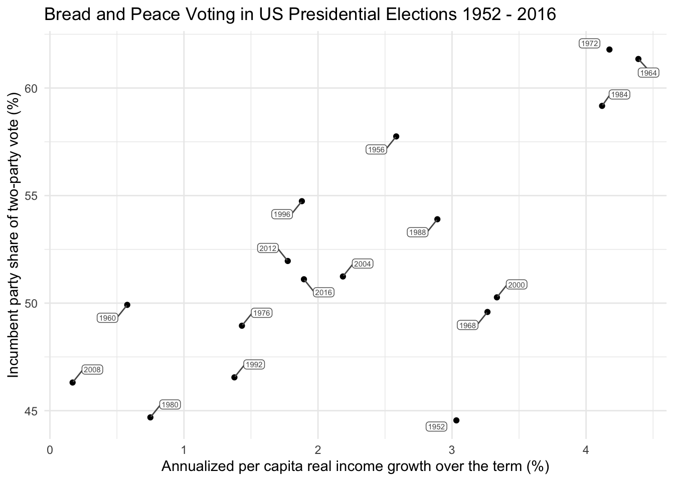
When two continuous variables are considered, a scatterplot is an excellent tool for visualization. It’s important to determine if the relationship appears linear (as opposed to curvilinear) and to note any possible outliers or other strange occurrences in the data.
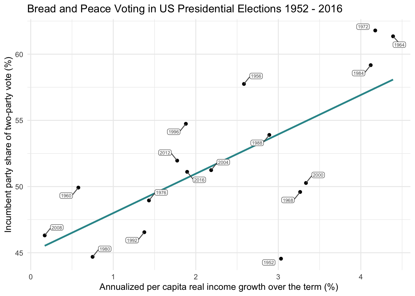
If we want to summarize the relationship between the variable on the x-axis (growth) and the variable on the y-axis (vote), one option is to draw a straight line through the data points. This is accomplished in the plot below via the geom_smooth() function — which adds a smoothed line, specifically a linear model (i.e., method = "lm", formula = y ~ x).
bp |>
  ggplot(mapping = aes(x = growth, y = vote)) +
  geom_point() +
  geom_smooth(method = "lm", formula = y ~ x, se = FALSE, color = "#2F9599") +
  ggrepel::geom_label_repel(mapping = aes(label = year),
                            color = "grey35", fill = "white", size = 2, box.padding =  0.4,
                            label.padding = 0.1) +
  theme_minimal() +
  labs(title = "Bread and Peace Voting in US Presidential Elections 1952 - 2016",
       x = "Annualized per capita real income growth over the term (%)",
       y = "Incumbent party share of two-party vote (%)")
This straight line does a reasonable job of describing the relationship between the predictor and the outcome. Many relationships can be explained with a straight line, and this is the primary purpose of a linear regression model. However, it is critical to note that imposing a straight line to describe the relationship between two variables is only appropriate if the relationship between the variables is indeed linear. A linear relationship means that a change in one variable is consistently associated with a proportional change in the other variable. In other words, if the points on the scatterplot appear to rise or fall at a steady rate, a straight line can adequately describe the trend. Otherwise, other, more complex, models need to be considered.
Examples of nonlinear relationships
The graphs below show a variety of scatterplots where X and Y are clearly related, but the pattern is nonlinear — that is, the data do not follow a consistent upward or downward trend that can be captured by a straight line.
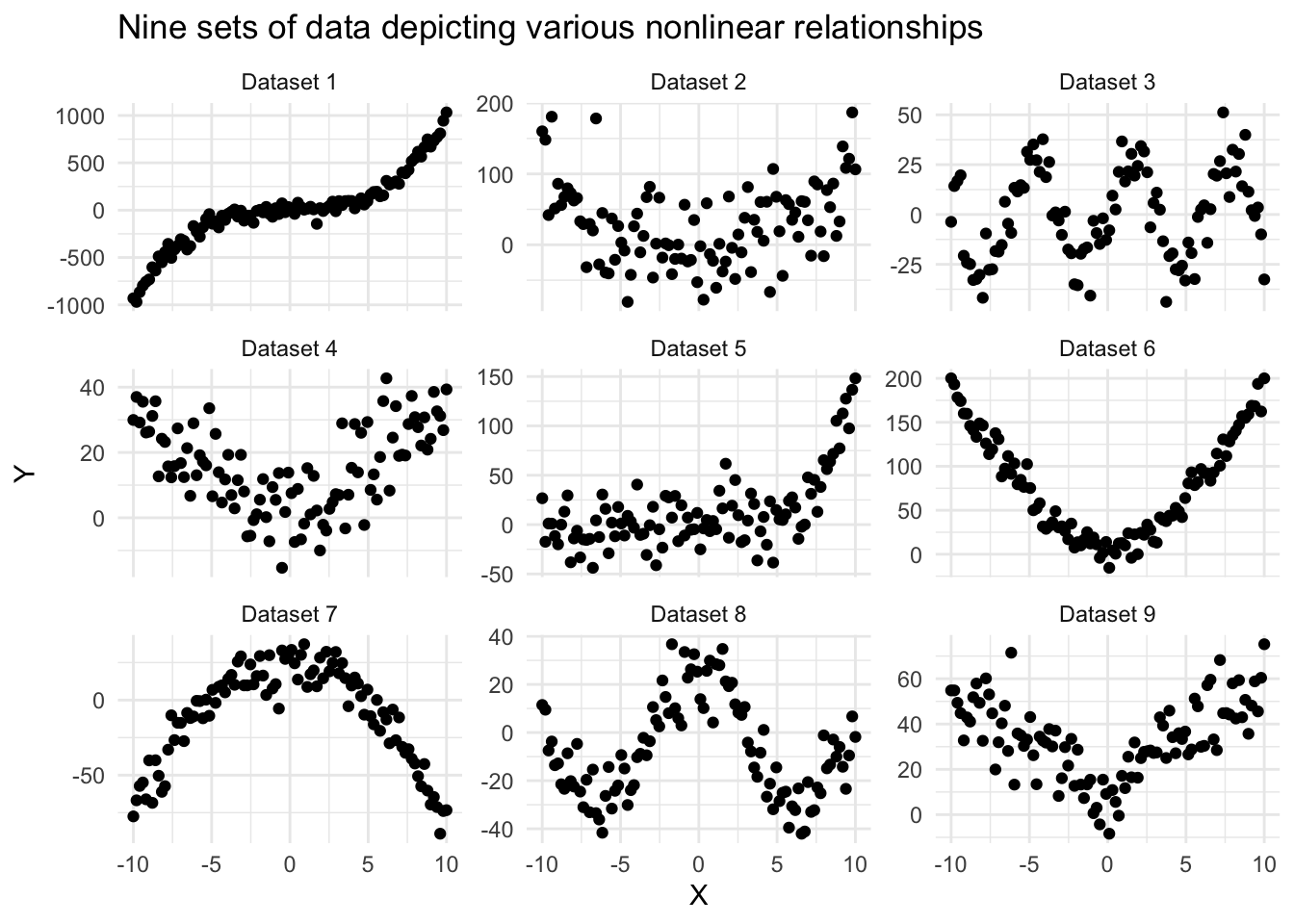
Each panel shows a different type of nonlinear relationship — from exponential growth and U-shaped curves to wave-like and piecewise patterns. In these cases, a simple linear regression model would not be appropriate, as it would fail to capture the true shape of the relationship.
When you encounter these kinds of patterns in your own data, you may need to consider alternative modeling approaches, such as:
Polynomial regression (to capture curves),
Log or exponential transformations of variables,
Nonlinear models (e.g., exponential or logistic functions),
Or even nonparametric methods like LOESS, which make fewer assumptions about the form of the relationship.
We’ll consider some of these types of models later in the course. The key takeaway: Always visualize your data first. Plotting X and Y together can help you determine whether a linear model is appropriate — or whether you’ll need a different tool to more accurately describe the relationship.
Understanding the Regression Line: Intercept and Slope
Before we dive into fitting a regression model, it’s important to build a strong intuitive understanding of what a regression line represents and how it helps us describe relationships between two continuous variables.
What is a regression line?
A regression line is a straight line we draw through a scatterplot of data to summarize the relationship between a predictor variable (X) and an outcome variable (Y). If a straight-line relationship is a good approximation of the data, we can describe the line using two key components:
The Intercept: This is the predicted value of Y when X = 0. It’s the point where the line crosses the y-axis.
The Slope: This tells us how much Y is expected to change for a one-unit increase in X.
Visualizing the intercept
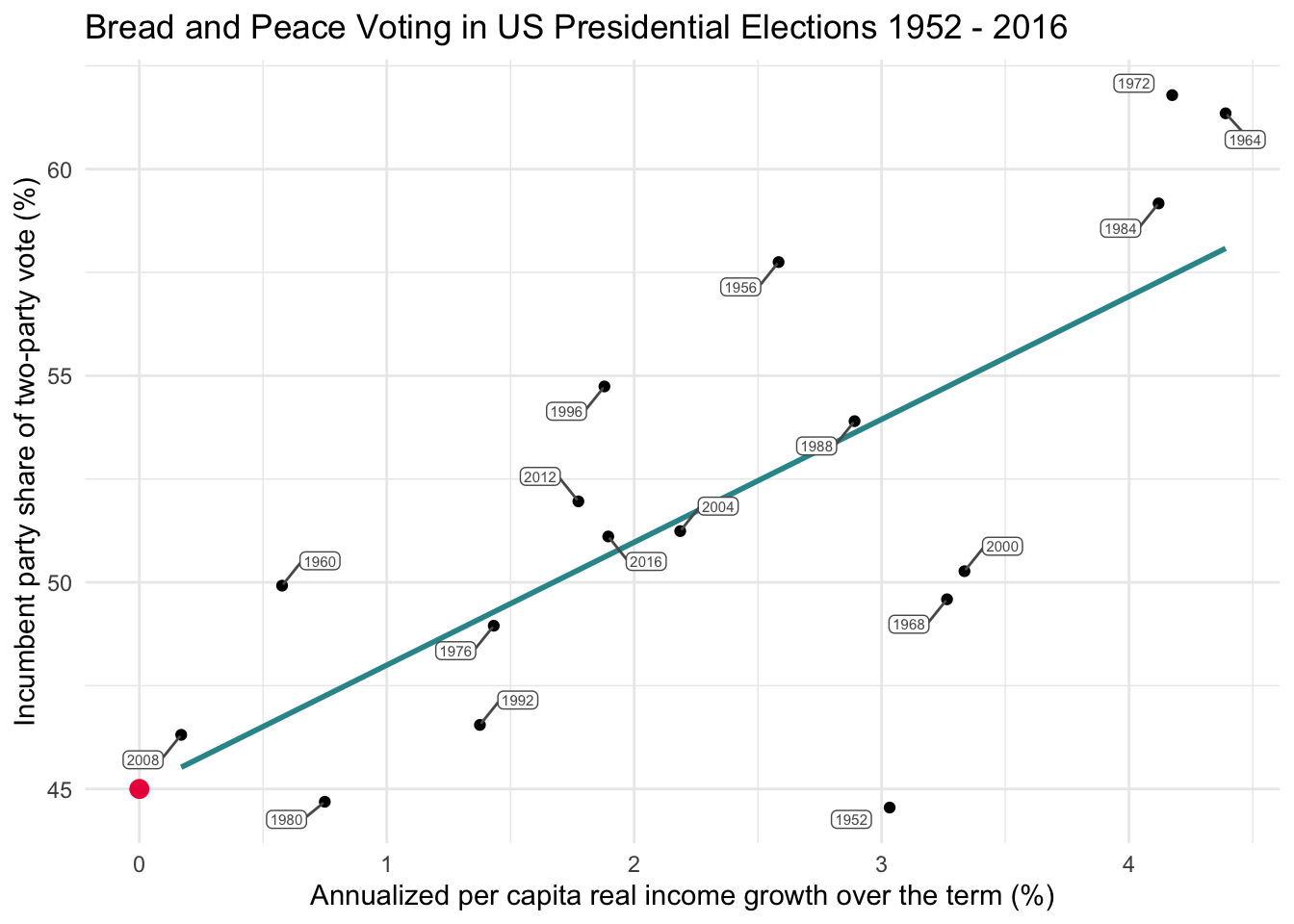
In our example, we’re modeling the relationship between income growth and vote share for the incumbent party in U.S. presidential elections. Even though no presidential election cycle in the data frame has 0% growth, we can still extrapolate the regression line to see what it would predict at \(x_i = 0\). On the graph below, a pink dot marks this intercept — suggesting that, if growth were 0%, the model predicts the incumbent would receive about 45% of the vote.
Visualizing the slope
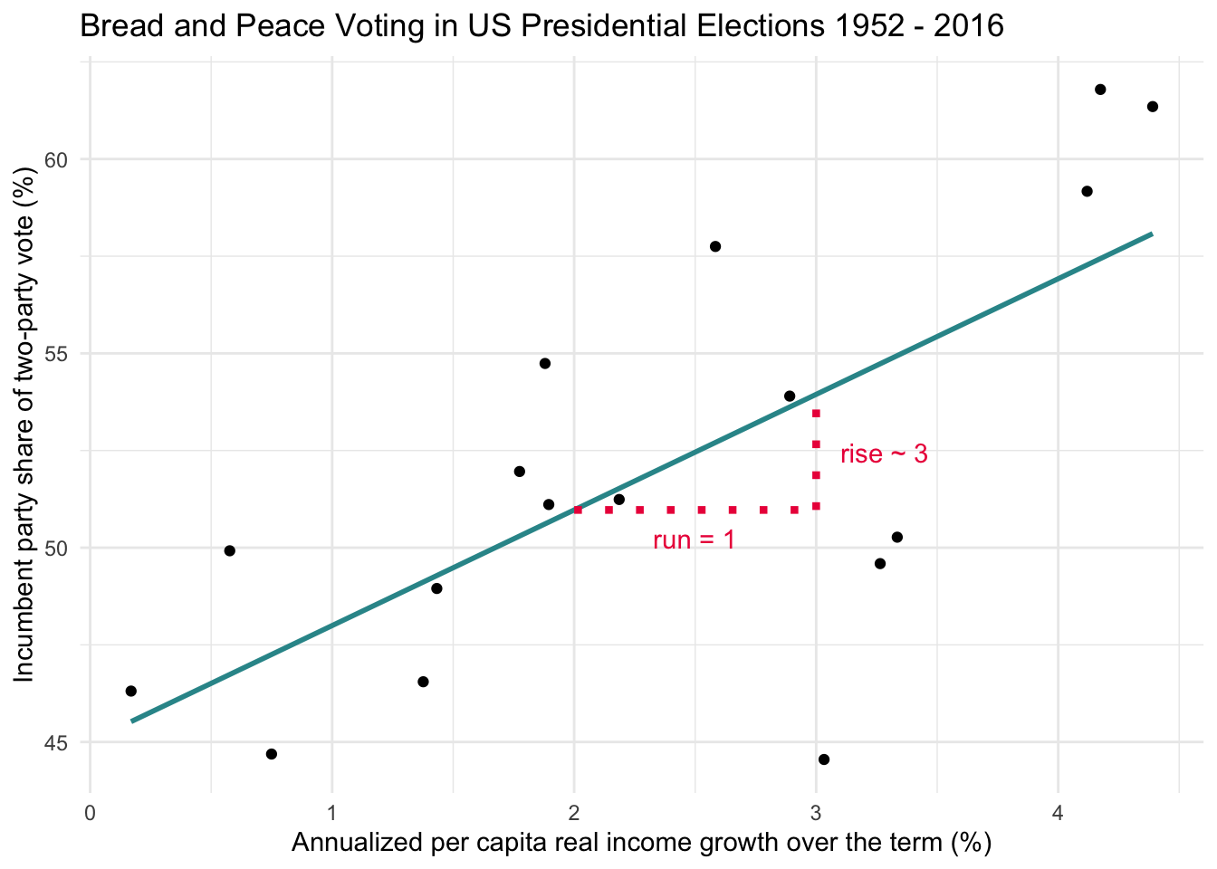
Now let’s focus on the slope—the heart of the regression line. The slope tells us how much the outcome variable (in this case, vote share) is predicted to change for each one-unit increase in the predictor variable (income growth).
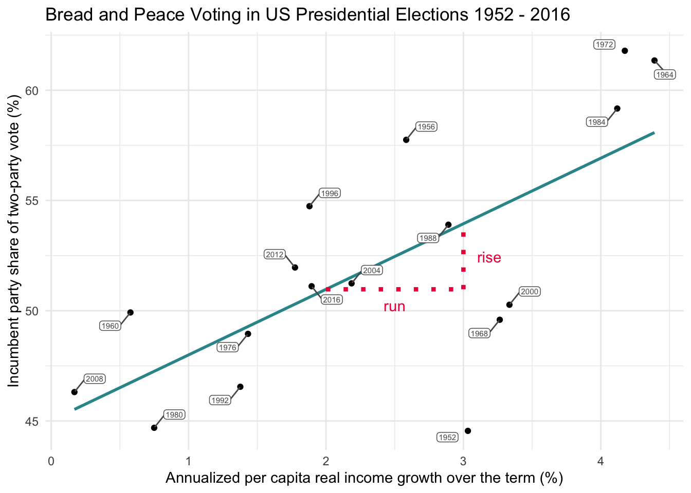
Let’s walk through a concrete example using the graph above. Suppose we look at what happens when income growth increases from 2% to 3%. This one-unit change on the x-axis is often called the run. The corresponding change on the y-axis — the predicted change in vote share — is called the rise.
To help visualize this, study the graph below, which depicts the same concept in a slightly different way. When growth = 2%, the regression line predicts the vote share will be 51%. When growth = 3%, the predicted vote share rises to 54%.
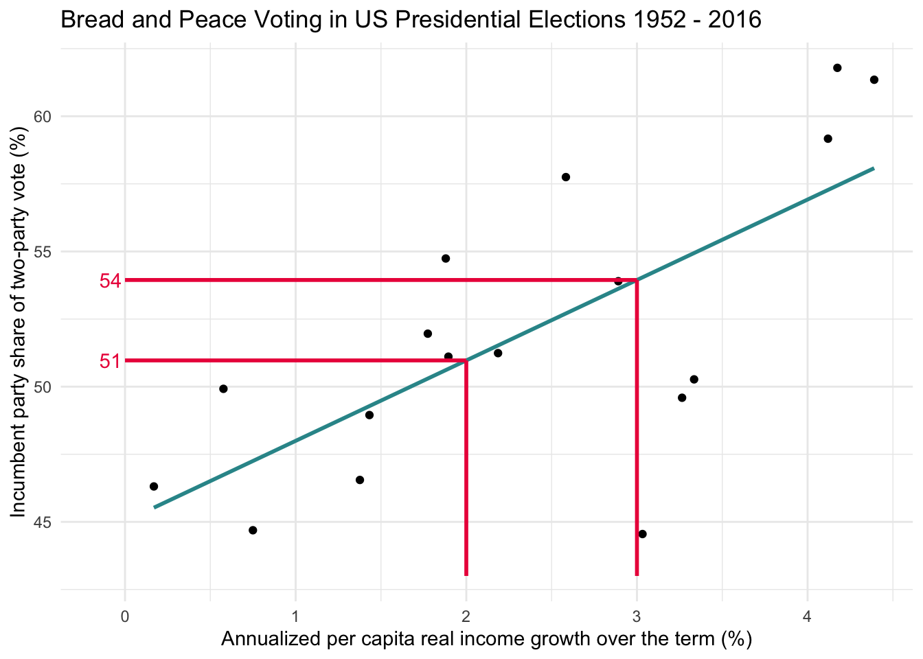
That’s a rise of 3 percentage points in vote share for a run of 1 percentage point in income growth. So, the slope — which is calculated as rise over run — equals:
\[ \text{slope} = \frac{\text{rise}}{\text{run}} = \frac{3}{1} = 3 \]
In plain language:
For each 1% increase in income growth, the model predicts that the incumbent party will gain about 3 percentage points in vote share.
This simple ratio — rise over run — is what defines the slope of the best-fitting line. Understanding this concept is key to interpreting what a regression model is telling us.
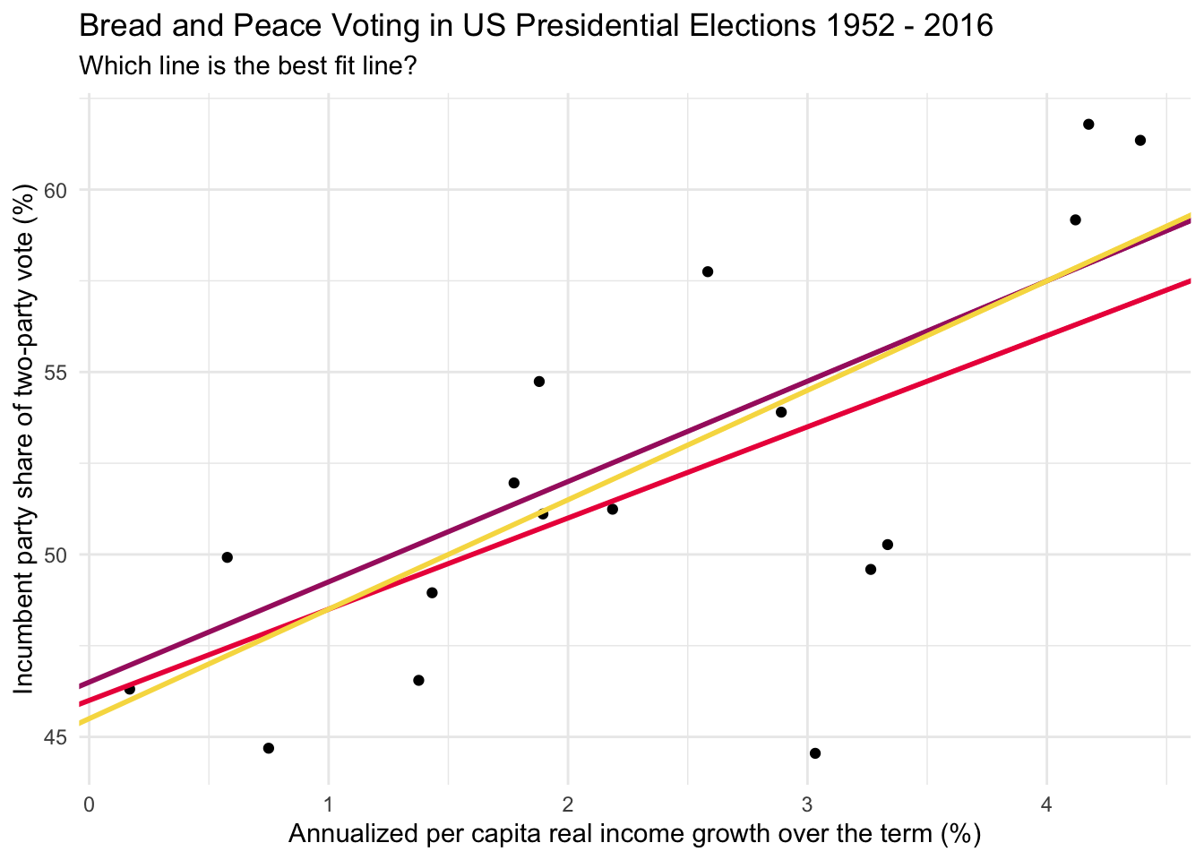
Why this line?
You might wonder: Why this line? Couldn’t we draw many different lines through the data points?
Absolutely. In fact, there are infinitely many possible lines. But we want the best-fitting one — the line that most accurately captures the pattern in the data. That’s where the least squares criterion comes in. We will study this method in the next part of this Module. If you’d like to build your intuition a bit more before studying the mathematics behind estimation of the best fit line — check out this engaging application.
Estimate the best fit line
We can imagine many reasonable lines that could be drawn through the data points to relate the predictor to the outcome. For example, each of the lines on the graph below seems reasonable.
How do we determine the best fit line for the data? For any given X and Y variable pair that are linearly related, there is indeed one best fitting line. The best fitting line is the line that allows the \(x_i\) scores (growth) to predict the \(y_i\) scores (vote) with the highest amount of accuracy.
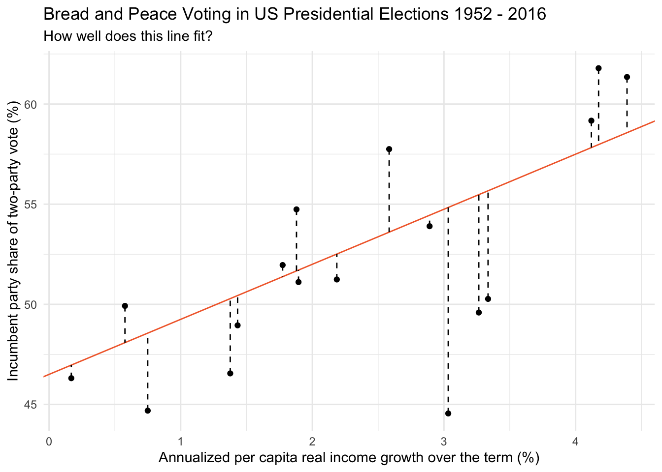
To find the best fit line, we use the least squares criterion. The least squares criterion dictates that the best fitting line is the line that results in the smallest sum of squared errors (or residuals). Here’s a simplified explanation of how least squares works:
Begin by plotting the data: Plot your two continuous variables on a scatterplot. One variable goes on the y-axis, and the other goes on the x-axis. Each point on the scatterplot represents an observation/case in your data frame.
Draw a line: Imagine drawing a line through the scatterplot. The line can be placed in an infinite number of ways, but we want to find the “best” way.
Calculate the distance from each point to the line you drew: For each point, calculate the vertical distance from the point to the line. See the graph below for a depiction. These distances are called residuals or prediction errors. Some of these will be positive (when the point is above the line), and some will be negative (when the point is below the line). This distance represents how “off” our prediction is for each point (i.e., the difference between a case’s observed score, and what we predict the case’s score to be given the drawn line).
Square each distance and add them up: Because negative and positive residuals cancel each other out, we square each distance, which makes all the distances positive, then add them together. This sum is called the Sum of Squared Errors (SSE) — also referred to as Sum of Squared Residuals1.
Adjust the line to minimize the sum: The best fit line is the one where this SSE is as small as possible. The method of finding this best fit line is called least squares because it minimizes the SSE.
In summary, the best fit line is found by minimizing the sum of the squared distances from each point to the line. This line represents the best linear approximation of the relationship between the two variables, assuming that the relationship is indeed linear.
Consider a few candidate lines
Let’s consider a few candidate lines.
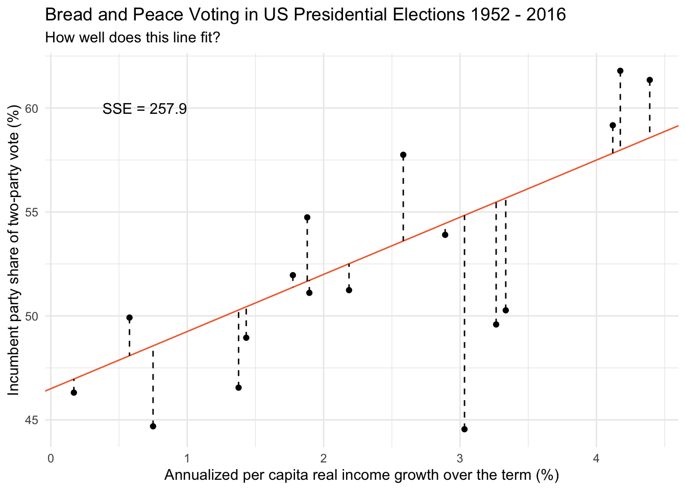
Candidate line #1
First, consider the line on the graph below as a candidate best fit line. This line has an intercept of 46.50 and a slope of 2.75.
Given this line, for each data point, we can calculate the election’s predicted score (the data point on the orange line given the election’s score on growth — which is recorded as predicted_score in the table below).
For example, find the data point for the 1956 election in the graph above. The coordinates for this election are x = 2.58, y = 57.75. If we drop straight down from this data point to our candidate line (in orange) — we see that the predicted score on the line corresponds to a vote share of 53.60. The difference between the observed vote share (57.75) and the predicted vote share (53.60) is 4.15.
The distance between each election’s predicted score and observed score represents it’s residual (the dashed lines on the graph). These are recorded in the table below under residual.
We then square each election’s residual to get the value in the table recorded as residual_sq. Then, we sum the squared residuals across all 17 elections to obtain the SSE for our candidate line.
| year | vote | growth | predicted_score | residual | residual_sq | |
|---|---|---|---|---|---|---|
| 1952 | 44.55 | 3.03 | 54.84 | −10.29 | 105.87 | |
| 1956 | 57.75 | 2.58 | 53.60 | 4.15 | 17.18 | |
| 1960 | 49.92 | 0.58 | 48.09 | 1.83 | 3.36 | |
| 1964 | 61.35 | 4.39 | 58.57 | 2.78 | 7.71 | |
| 1968 | 49.59 | 3.26 | 55.48 | −5.89 | 34.66 | |
| 1972 | 61.79 | 4.17 | 57.98 | 3.81 | 14.52 | |
| 1976 | 48.95 | 1.43 | 50.44 | −1.49 | 2.22 | |
| 1980 | 44.69 | 0.75 | 48.56 | −3.87 | 14.99 | |
| 1984 | 59.17 | 4.12 | 57.83 | 1.34 | 1.80 | |
| 1988 | 53.90 | 2.89 | 54.45 | −0.55 | 0.30 | |
| 1992 | 46.55 | 1.38 | 50.29 | −3.74 | 13.95 | |
| 1996 | 54.74 | 1.88 | 51.67 | 3.07 | 9.43 | |
| 2000 | 50.27 | 3.33 | 55.67 | −5.40 | 29.17 | |
| 2004 | 51.24 | 2.19 | 52.51 | −1.27 | 1.62 | |
| 2008 | 46.31 | 0.17 | 46.97 | −0.66 | 0.43 | |
| 2012 | 51.96 | 1.77 | 51.38 | 0.58 | 0.34 | |
| 2016 | 51.11 | 1.90 | 51.71 | −0.60 | 0.36 | |
| SSE = ∑ | — | — | — | — | — | 257.90 |
The SSE for this candidate line is 257.90.
Candidate line #2
Now, let’s consider the mean of Y as a potential line. Here the intercept is the mean of vote (51.99) and the slope is 0.00.
Clearly, this line is not so great in explaining the relationship between the two variables — the SSE is very large (473.67).
Candidate line #3
How about the best fit line recorded by ggplot2 using the geom_smooth() function? This is depicted in the graph below. The intercept (recorded to three decimal places) is 45.021 and the slope is 2.975.
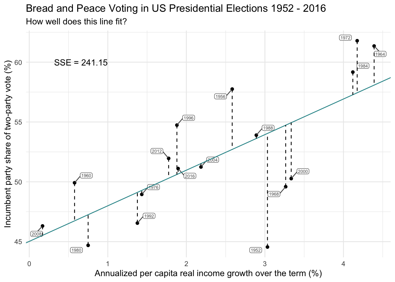
For this line, the SSE is 241.15 — the lowest we’ve seen so far. This is our best-fitting line.
As expected, when we use method = "lm" within the geom_smooth() function in our ggplot() call — along with formula = y ~ x — R fits a linear model predicting vote from growth. This overlays the least squares regression line, which minimizes the SSE. The graph below displays this best fit line.
bp |>
  ggplot(mapping = aes(x = growth, y = vote)) +
  geom_point() +
  geom_smooth(method = "lm", formula = y ~ x,  se = FALSE, color = "#2F9599") +
  ggrepel::geom_label_repel(mapping = aes(label = year),
                            color = "grey35", fill = "white", size = 2, box.padding =  0.4,
                            label.padding = 0.1) +
  theme_minimal() +
  labs(title = "Bread and Peace Voting in US Presidential Elections 1952 - 2016",
       subtitle = "Best fit line shows how income growth predicts incumbent party vote share",
       "Annualized per capita real income growth over the term (%)",
       x = "Annualized per capita real income growth over the term (%)",
       y = "Incumbent party share of two-party vote (%)")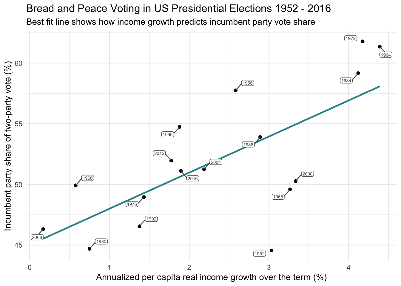
An equation for the best fit line
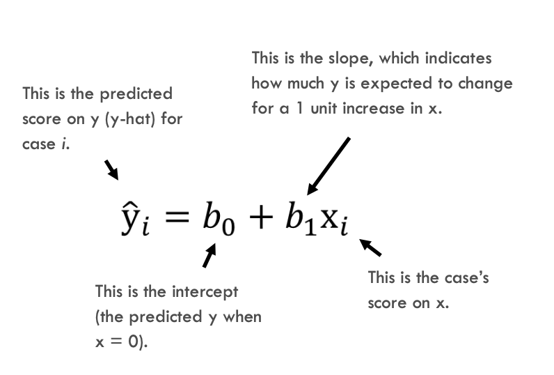
The best fit line is defined by an equation consisting of:
An intercept: The predicted value of vote when growth = 0.
A slope: The predicted change in vote for each one unit increase in growth. This equation is depicted below. For this depiction, the Y and X scores for each election year are subscripted with an i to denote that each case (i.e., election year in our example) has a score for \(y_i\) and a score for \(x_i\).
The best fit line for our Bread and Peace data is represented by the following equation. The intercept, that is, the predicted score for vote when growth = 0, is 45.021. The slope, that is, the predicted change in vote for each one unit increase in growth, is 2.975.
\[ \hat{y_i} = b_{0}+b_{1}x_i \]
\[ \hat{y_i} = 45.021+2.975x_i \]
You may also see the equation for a line written as \(\hat{y}_i = mx_i + b\), where \(b\) is the intercept (equivalent to \(b_0\)) and \(m\) is the slope (equivalent to \(b_1\)). These are just different notations for the same concept.
Also, notice the hat over the \(y_i\) in \(\hat{y}_i\). This symbol indicates a predicted (or fitted) value based on the regression equation. It’s our model’s best guess for what the outcome would be, given a specific value of growth.
Predicted scores based on the equation
Let’s use this equation to obtain predicted scores.
The 1988 election
We’ll start with the 1988 election.

In this election, George Bush Sr. ran against Michael Dukakis. Coming off of Ronald Reagon’s second term, Bush was the incumbent party candidate. The economy was in pretty good shape, income growth was 2.89%. Using our equation, we’d predict Bush to garner about 53.6% of the vote share.
\[ \hat{y_i} = b_{0}+b_{1}x_i \] \[ \hat{y_i} = 45.021+2.975x_i \]
\[ \hat{y_i} = 45.021+(2.975\times2.89)=53.62 \]
Take a look at the graph below, we see that this prediction (marked with an orange dot) is very close to what Bush actually garnered (53.90% — see the dot marked with the label 1988). That is, for this election, the Bread and Peace Model does an excellent job of predicting the election results. (Note that I changed the best fit line to a dashed gray line to help you see the orange dot).
In this way, we can hand calculate the predicted score (also referred to as the fitted value or y-hat or \(\hat{y}\)) for every case in the data frame. Doing so yields the table below. The column labeled .fitted provides the predicted score for every election year.
Important
To practice and solidify this concept in your mind, please use the equation above to calculate the predicted score by hand for a few of the years.
The 1968 election
Let’s consider another example — the 1968 election between Hubert Humphrey (Democrat) and Richard Nixon (Republican).

Humphrey was the incumbent and the US was in the midst of the Vietnam War. During Humphrey’s term, economic growth was 3.26%, he only secured 49.59% of the vote, and ultimately lost to Nixon. Based on our best fit line, we would have predicted Humphrey to receive 54.73% of the vote.
\[ \hat{y_i} = 45.021+(2.975\times3.26)=54.73 \]
This predicted score is marked by the orange dot in the graph below and labeled \(\hat{y_i}\). Humphrey’s actual vote total (see the point marked with the label 1968) was much poorer than our best fit line would have predicted — that is, given the relatively good economy, he did not perform nearly as well as we would have expected based on our linear model. To illustrate this point, I connected the predicted and observed score for vote for the 1968 election with a dotted black line in the graph below.

Residual scores based on the equation
So far, we’ve seen that every case in the data frame has an observed outcome score (\(y_i\)) — which is the variable called vote in our example. We’ve also learned that, based on the equation for the best fit line, we can compute the predicted outcome (i.e., the fitted value or \(\hat{y_i}\)) for every case in the data frame.
Additionally, using the observed score and the predicted score for each case, we can calculate each case’s residual. The residual, denoted \(e_i\), is simply the difference between a case’s observed score and their predicted score:
\[ e_i = y_i - \hat{y}_i \]
Specifically, we subtract each case’s predicted score from their observed score. The residual is denoted by \({e_i}\) in the figure below. For the 1968 election, the residual is -5.14 (calculated as 49.59 - 54.73).
In the same way that we calculated the predicted score (.fitted) for each case, we can also calculate the residual for each case. These are all displayed in the table below, under the column .resid. Note the calculated fitted value and the residual for the 1968 election — and match them up to the work we just did to compute them.
Important
To solidify these concepts, please calculate a few predicted scores and residuals for election years yourself, and map them onto the graph above.
We can write an alternative version of our regression equation that incorporates the residual:
\[ {y_i} = b_0 + b_1x_i + e_i \]
Here, we replace \(\hat{y_i}\) with the actual observed score (i.e., \({y_i}\)), and we add the case’s residual (represented as \({e_i}\)). In this way, the actual observed score for Y for each case can be calculated using the intercept and slope for the best fine line (to obtain \(\hat{y_i}\)) and adding the case’s residual score. For example, to reproduce the observed score for vote (\({y_i}\)) for 1952, we use the following equation: \[{y_i} = 45.021 + (2.975\times3.03) + (-9.49) = 44.55\]
Important
Please use the same technique to recover vote for a couple additional years to be sure you understand where the numbers come from.
At this point, you might be worried about the time and energy needed to test a whole lot of lines in order to find the one that results in the smallest sum of squared errors — and then to hand compute fitted values and residuals. Fortunately, R can solve for the best fine line and compute these new values for us. We’ll walk through how this is done in the next section.
Fit a simple linear regression model
The lm() function in R is used to fit a linear model. In the code below I first define the name of the R object that will store our linear model results (bp_mod1). Then, I specify the desired equation in the lm() function. We want to regress the outcome (i.e., the \(y_i\) scores) on the predictor (i.e., the \(x_i\) scores), that is, we want to regress vote on growth to determine if growth can predict vote. This is coded in the lm() function by writing vote ~ growth. Think of the tilde in this instance as saying “regressed on.” We also need to indicate the data frame to use.
bp_mod1 <- lm(vote ~ growth, data = bp)Obtain the regression parameter estimates
The tidy() function from the broom package is used to view the regression parameter estimates (i.e., the intercept and the slope). The package has a number of functions that we’ll use — they focus on converting the output of various statistical models in R into tidy data frames. That is, broom provides functions that tidy up the results of model fitting, making it easier to work with and analyze the results using other tidyverse tools.
To use the tidy() function to see the regression results, we just need to pipe in the R object that we designated to store our linear model results (bp_mod1).
bp_mod1 |>
  tidy() |>
  select(term, estimate)
For now, we are only going to be concerned about the first two columns of the tidy output — the columns labeled term and estimate. To avoid distractions, I’ve extracted just these two columns (we’ll consider the other columns produced by tidy() later in the course). Let’s map these estimates onto our equation. The term labeled intercept provides the intercept of the regression line and the term labeled growth provides the slope of the regression line.
\[ \hat{y_i} = b_{0}+b_{1}x_i \]
\[ \hat{y_i} = 45.021+2.975x_i \]
These estimates are interpreted as follows:
The intercept is the predicted value of \(y_i\) when \(x_i = 0\), therefore, it is the predicted vote percentage for the incumbent party when growth in income equals 0%.
The slope is the predicted change in the \(y_i\) scores for each one unit increase in the \(x_i\) scores. That is, for each one percentage point increase in growth (e.g., going from 1% to 2%, or 2% to 3%), we expect the percent of vote share garnered by the incumbent party, vote, to increase by 2.975 percentage points.
Obtain the predicted values and residuals for each case
We can obtain the predicted values and residuals using the augment() function from the broom package. In the code chunk below, bp_mod1 (the object holding our model results) is piped into the augment() function — this function augments the data frame with additional information from the linear model — including the predicted values (.fitted) and the residuals (.resid). As you’ll learn later in the course, the augment() function adds more information than just these values — it also adds numerous statistics for assessing the assumptions of the linear regression model. Since we won’t be concerned about these until later in the course, the select() function from dplyr is used to select only the columns that we need for now.
bp_mod1 |>
  augment(data = bp) |>
  select(year, vote, growth, .fitted, .resid)
Obtain the overall model summary
We can also obtain additional summary information about the overall model using the glance() function from broom.
bp_mod1 |>
glance() |>
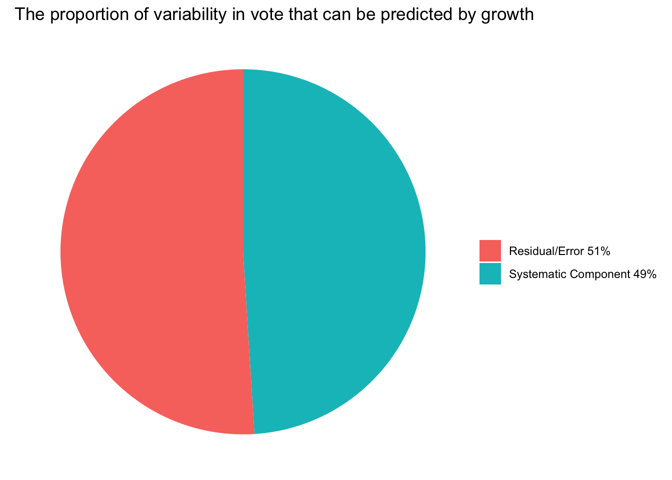
select(r.squared)For now, we’ll only be concerned about the r.squared column. This value is 0.0491. It represents a commonly considered term in regression modeling called R-squared or \(R^2\). \(R^2\) is the proportion of the variability in the outcome (vote in our example) that is explained by the predictor (growth in our example).
It is calculated by considering the amount of variability explained by our model (the systematic part of the model), and the amount not explained by our model (the error, also called the residual).
The systematic part is often called the Sum of Squares Regression (SSR) — and is calculated by taking the difference between the predicted Y for each case (\(\hat{y_i}\)) and the mean of Y (\(\bar{y}\)), squaring it, and then summing across all cases in the sample. In equation form this is \(SSR = Σ(\hat{y_i} – \bar{y})^2\). Note that Σ, the Greek letter called sigma, means to sum. SSR represents how much our predictor can move our prediction away from simply predicting the average outcome (\(\bar{y}\)) for every observation (which is what we would do if we had no predictors at all). In other words, SSR captures how much better our model’s predictions are than just predicting the average outcome (e.g., average vote, (\(\bar{vote}\))).
The error part is often called the Sum of Squares Error (SSE) — and is calculated by taking the difference between the predicted Y for each case (\(\hat{y_i}\)) and the observed Y for each case (\(y_i\)) (which is the residual), squaring it, and then summing across all cases in the sample. In equation form this is \(SSE = Σ({y_i} - \hat{y_i})^2\). As mentioned earlier, the goal of a linear regression model is to create a line that best fits the data, which means it minimizes the differences between observed values and predicted values. However, no model is perfect, and there will always be some level of error. These errors in prediction are the differences between the observed values and the fitted/predicted values. The SSE gives us a single measure of the total error of the model’s predictions. So, the SSE essentially represents the unexplained variance in the outcome variable.
To further build our intuition, let’s calculate these quantities with some code.
First, lets compute the needed quantities for each case — that is, the squared difference between the predicted \(y_i\) and the mean of of the \(y_i\) scores for SSR and the squared residual (for SSE).
get_rsq <-
  bp_mod1 |>
  augment(data = bp) |>
  mutate(for_SSR = .fitted - mean(vote), # calculate the difference between each predicted score and the mean of y
         for_SSR2 = for_SSR^2) |>  # square the difference
  mutate(for_SSE2 = .resid^2) |>  # square the residual
  select(year, vote, growth, .fitted, .resid, for_SSR, for_SSR2, for_SSE2)
get_rsq
Now, we can sum the squared quantities that we just calculated across all cases (all 17 elections).
SSR_SSE <- get_rsq |>
  summarize(SSR = sum(for_SSR2),
            SSE = sum(for_SSE2))

SSR_SSE
Finally, to calculate the \(R^2\), we take SSR divided by the sum of SSR and SSE. This denominator is also called Sum of Squares Total (SST) as it represents the total variability in the outcome.
\[ R^2 = \frac{\text{SSR}}{\text{SSR} + \text{SSE}} \]
SSR_SSE |>
  mutate(r_squared = SSR/(SSR + SSE))
Of course, this is the same value of \(R^2\) that glance() calculated for us. You can multiply the proportion by 100 to express it as a percentage, which indicates that about 49% of the variability in the share of the vote received by the incumbent party is explained by the income growth that US residents achieved during the prior term. The remaining 51% might be just random error in the model, or this remaining variability might be accounted for by other variables. For example, in Module 11 we will determine if additional variability in vote can be accounted for by adding fatalities (i.e., loss of U.S. military troops) as an additional predictor to the regression model. Hibb’s Bread and Peace Model asserts that it should.
Recall from the beginning of the Module, we learned that an outcome can be modeled as:
\[\text{Outcome} = \text{Systematic Component} + \text{Residual}\]
And, that statistical techniques allow us to explain variation in our outcome (the systematic component) in the context of what remains unexplained (the residual). The \(R^2\) gives us the quantity of the systematic component — the proportion of the variance in vote that can be predicted by growth. The pie chart below depicts this for our example.
The \(R^2\) is very useful, but it’s important to recognize that it has limitations. While a higher \(R^2\) value indicates more of the variability in the outcome can be predicted by the predictor, it does not necessarily mean the model is good. A model can have a high \(R^2\) value but still be a poor predictive model if it’s overly complex (overfitting) or if key assumptions of the regression analysis are violated. These are topics we will discuss later in the course.
The standard error of the residual
There is one other output from glance() that is of interest to us now — and that is sigma, also referred to as the residual standard error.
bp_mod1 |>
  glance() |>
  select(sigma)
Sigma (\(\sigma\)) represents the standard deviation of the residuals. Ideally, we want to compare \(\sigma\) to the standard deviation of the outcome variable, Y. Our goal is that after accounting for the predictors, the standard deviation of the residuals (\(\sigma\)) is smaller than the standard deviation of Y. This reduction would indicate that the predictor (or predictors in the case of a multiple linear regression) provides meaningful information to predict the outcome.
\[SD_y = \sqrt{\frac{\sum (y_i - \bar{y})^2}{n-1}} = 5.44\]
\[SD_{y|x} = \sqrt{\frac{\sum (y_i - \hat{y})^2}{n-2}} = 4.01\]
The illustration below captures this concept. On the graph’s left side, you’ll see a large distribution titled “full distribution of y.” Taking the outcome vote, as an example, this wide spread showcases the complete variability of the variable vote. The standard deviation of the outcome, which is the square root of its variance, measures this spread and is calculated without considering any predictors.
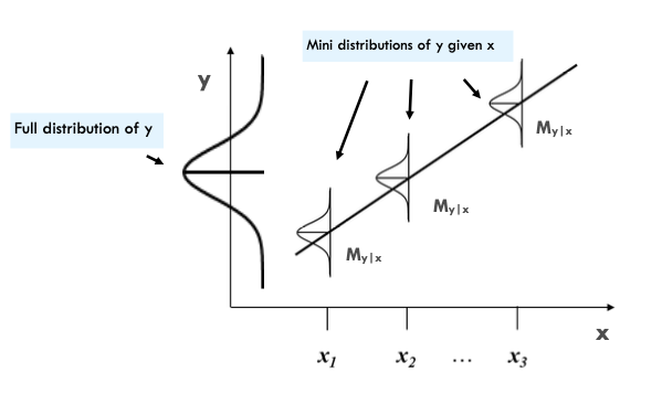
Contrasting this, when we introduce a predictor, we aim for the smaller distributions of the \(\hat{y_i}\) scores given distinct values of \(x_i\) to be narrower than the overall distribution of the \({y_i}\) scores. If these smaller distributions are indeed narrower, it reaffirms that the predictor is providing significant insights into the prediction of the outocme.
Use the equation to forecast
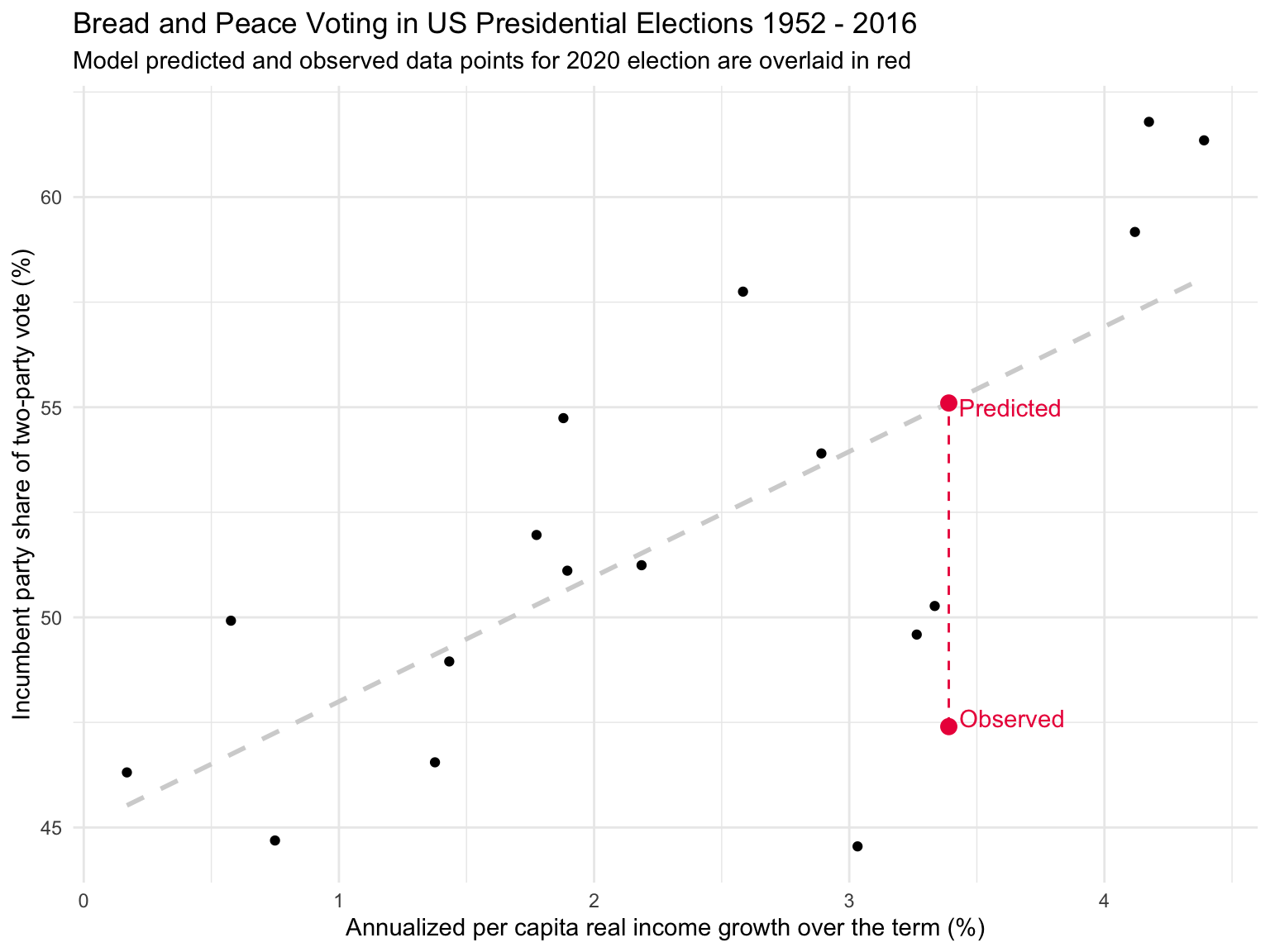
We can use our equation to forecast “out of sample” predictions. That is, predict what might happen for years not included in the data frame based on the fitted model. For example, 2020 and 2024 data was not included in Thomas’s data frame that we analyzed.
Let’s consider the 2020 election between Donald Trump (Republican — the incumbent) and Joe Biden (Democrat). I applied the same method in the Thomas paper to calculate growth for the Trump term ending in 2020 — and obtained an estimate of 3.39. We can plug this number into the equation that we obtained using years 1952 to 2016 to get a predicted score for vote.
\[\hat{y_i} = 45.021+(2.975\times3.39) = 55.11\]
This forecast means that, based on income growth alone, we would have expected Donald Trump to garner about 55.1% of the vote share. There were 81,285,571 votes cast for Biden and 74,225,038 votes cast for Trump in the 2020 election. Thus, the actual vote score for the 2020 election (i.e., the percentage of votes garnered by the incumbent candidate) was 47.7%, producing a residual of about -7.4. The graph below overlays the 2020 data point onto our graph.
Building a regression model and using it to forecast future outcomes can be an incredibly valuable technique. By identifying and quantifying the relationship between variables based on historical data, we can make informed predictions about what might happen under similar conditions in the future. This is the cornerstone of many fields, including finance, economics, medicine, and machine learning, to name just a few.
Correlation
For two numeric variables (e.g., vote and growth in the Bread and Peace data frame) we can also calculate the correlation coefficient. A correlation coefficient, often abbreviated as \(r\), quantifies the strength of the linear relationship between two numerical variables using a standardized metric. A correlation coefficient ranges from -1 to 1, where -1 indicates a perfect negative relationship (as one value increases, the other decreases), and +1 indicates a perfect positive relationship (as one value increases, the other increases). A correlation coefficient of 0 indicates no relationship between the two variables. A correlation coefficient captures how tightly knit the data points are about the best fit line and the direction of the line.
To grow your intuition for correlation coefficients, check out this interactive application.
The correlate() function in the corrr package calculates the correlation coefficient and puts it in a nice matrix form. Note that a correlation matrix displays the correlations between each pair of variables in a data frame. The correlations are listed in both the upper and lower diagonals to provide a symmetrical representation.
bp |>
  select(growth, vote) |>
  corrr::correlate()
Correlation computed with
• Method: 'pearson'
• Missing treated using: 'pairwise.complete.obs'The correlation between vote and growth is 0.70, denoting a strong, positive association. Of note, the square of the correlation coefficient equals the \(R^2\) in a SLR (i.e., \(0.70^2 = 0.49\)).
While the unstandardized regression slope is expressed in the units of the Y variable, it depends on the units of both X and Y. Specifically, it tells us how much Y is expected to change (in its original units) for a one-unit increase in X. This gives us a sense of the magnitude and direction of the effect of X on Y, but the interpretation is tied to how X and Y are measured.
In contrast, the correlation coefficient is unitless — it describes the strength and direction of a linear relationship between two variables in standardized units. It tells us how closely the data cluster around a straight line, but not how steep that line is in the original measurement units.
Standardized regression equation
An interesting property of simple linear regression is that if we first convert both X and Y into z-scores, then fit a linear regression model, the slope of that model will equal the correlation coefficient. You can confirm this in the code below by looking at the estimated slope — it matches the correlation between vote and growth.
This means the correlation coefficient can also be interpreted as:
“The expected change in standardized Y for a one standard deviation increase in X.”
In this standardized model, the intercept is always 0. This is because, after standardization, both variables have a mean of 0. When the predictor (\(x_i\)) is 0 (i.e., exactly average), the predicted value of the outcome (\(\hat{y}_i\)) must also be 0 — which is exactly the mean of the standardized outcome variable. So the line must pass through the origin of the standardized coordinate system. That is, in any regression equation, the line is constructed so that when X is at its mean, the predicted value of Y is also at its mean. This is built into the mathematics of least squares regression. So when both X and Y have been standardized (i.e., have means of 0), the regression line must pass through the point (0, 0), making the intercept equal to 0.
bp_z <- bp |>
  select(vote, growth) |>
  mutate(vote_z = (vote - mean(vote))/sd(vote)) |>
  mutate(growth_z = (growth - mean(growth))/sd(growth))

bp_mod_z <- lm(vote_z ~ growth_z, data = bp_z)

bp_mod_z |>
  tidy() |>
  select(term, estimate) |>
  mutate(across(where(is.numeric), ~round(., 3)))
Note: the extra code below tidy() in the code above rounds the numeric estimates to three decimal places, making it easier to read. Otherwise, it would be printed out using scientific notation.
Correlation quantifies the strength and direction of a relationship between two variables. As we learned in this Module, estimating the relationship between two variables can be extremely useful. However, it is critical to realize that finding a relationship or correlation between two variables does not mean that one variable causes the other variable. That is, correlation does not equal causation. Causation indicates that one event is the result of the occurrence of another event — in other words, that one event causes the other. We’ll learn more about correlation and causation in psychological studies later in the course.
For now, please watch the following Crash Course Statistics video that introduces these issues.
Learning Check
After completing this Module, you should be able to answer the following questions:
- What does simple linear regression model, and when is it appropriate to use?
- What do the intercept and slope represent in a regression equation?
- How do you interpret the slope in a real-world context?
- What is the formula for a predicted value (\(\hat{y}_i\)), and how is it used?
- How is a residual (\(e_i\)) calculated and interpreted?
- What does the least squares criterion do when fitting a regression line?
- How can you determine if a linear model is appropriate by looking at a scatterplot?
- What does the \(R^2\) value tell us about the fit of a regression model?
- How is the correlation coefficient related to \(R^2\) in simple linear regression?
- Why does correlation not imply causation, and how can regression be misinterpreted in this way?
Footnotes
- You’ll also hear this quantity referred to as the Error Sum of Squares (or the Residual Sum of Squares) in other settings.