library(skimr)
library(gtsummary)
library(gt)
library(here)
library(tidyverse)Understanding Populations through Sampling and Descriptive Statistics
Module 7
Learning Objectives
By the end of this Module, you should be able to:
- Distinguish between a population and a sample and explain why sampling is important in research
- Describe the benefits and key principles of random sampling
- Discuss common challenges associated with survey research, such as non-response and sampling bias
- Efficiently compute descriptive statistics using R functions
- Apply the gtsummary package to create publication-ready tables for summarizing data
- Interpret and construct cross-tabulations to analyze relationships between categorical variables
- Create and interpret histograms and density plots to visualize distributions of quantitative variables
- Replicate descriptive stastistics findings from published research
- Explain how complex survey sampling designs (e.g., stratification, clustering, weighting) affect population-level estimates
Overview
Scientific research typically aims to achieve one or more of the following objectives: description, prediction, or causal inference. Each goal necessitates distinct methodologies concerning study design, data collection, and analysis. These points are well articulated by Dr. Ellen Hamaker and colleagues in this paper.
Description involves observing and characterizing phenomena as they naturally occur, without attempting to influence the outcomes. This approach often answers “what” is happening within a given context and relies heavily on data collection techniques like surveys and observational studies. For example, a Cognitive or Industrial Organizational Psychologist might explore the prevalence of Alzheimer’s disease among older adults in the U.S., and examine potential differences as a function of occupation. This descriptive analysis helps establish patterns or relationships between variables but does not imply causation. That is, if differences in the prevalence of Alzheimer’s disease across different occupations is observed in the descriptive statistics — this does not provide evidence in itself that certain occupations cause (or prevent) Alzheimer’s disease.
Prediction focuses on forecasting future outcomes based on existing data. This requires models that utilize historical data to predict future events or states. Such models are particularly valuable in scenarios where predicting an outcome can lead to early intervention or improved decision-making. For instance, a Clinical Psychologist might be interested in finding the key predictors of therapeutic alliance between a client and a practitioner. It’s important to note however that establishing a certain variable as a reliable predictor of a certain outcome does not provide evidence in itself that the predictor causes the outcome.
Causal Inference seeks to determine the causal effect of one variable on another, establishing a cause-and-effect relationship. This goal surpasses mere description (as in descriptive studies) or correlation (as in predictive studies) by aiming to demonstrate that changes in one variable directly result in changes in another. Experimental designs, especially randomized controlled trials (RCTs), are considered the gold standard for causal inference because they ensure that no background or pre-treatment variables are related to treatment assignment. For instance, a Health Psychologist may use an RCT to evaluate a new behavioral intervention for quitting smoking, ensuring any observed effects are due to the intervention itself. In cases where variables cannot be ethically or practically manipulated, such as naturally occurring exposures, researchers must rely on observational studies. These studies are more susceptible to confounding variables (variables that cause both the exposure and the outcome), which can bias results. To address this, researchers use techniques like stratification, matching, and statistical models to adjust for potential confounders. For example, an epidemiologist might use longitudinal data to study the impact of air pollution on respiratory health, adjusting for confounders like age, smoking habits, and socio-economic status to more accurately estimate the causal effect. In summary, while RCTs are ideal for establishing causality by controlling for confounding variables, observational studies require rigorous methods to mitigate confounding and achieve valid causal inferences.
Throughout the course, we will explore each of these research goals in depth, utilizing various data types and research designs. By understanding the strengths and limitations of each approach, you will be better equipped to choose appropriate methods for your research questions and critically assess the research of others. This foundational knowledge not only enhances your analytical skills but also prepares you for more advanced topics in modeling and statistical inference, which we will cover in upcoming Modules.
In this Module, we delve into descriptive statistics. This involves summarizing datasets to uncover patterns and insights that inform our understanding of a subject.
Introduction to Descriptive Statistics
In data analysis, descriptive statistics is a critical tool for understanding and interpreting data. It provides methods for gathering, summarizing, and reporting essential information about a population, helping to identify underlying patterns and inform effective solutions. Descriptive statistics is fundamental to research in the social and behavioral sciences, serving as the initial step in data interpretation.
For example, a scientist studying disease prevention may use descriptive statistics to:
Determine the prevalence of a disease
Monitor its trends over time
Identify demographic groups at higher risk.
These straightforward summaries offer a clear overview of the data, uncovering valuable insights about the population under study.
Survey Research
We’ll explore descriptive statistics through the lens of survey research — a widely used method for collecting data from a sample to infer characteristics of a population. Surveys, conducted via questionnaires, interviews, or digital tools, efficiently gather both quantitative and qualitative data at scale.
The United States routinely conducts large-scale national surveys to monitor the physical and mental health of its population. These publicly available data frames offer a valuable resource for researchers — ideal for exploring meaningful research questions, practicing data science skills, and even serving as the foundation for conference posters or publishable papers. Here are a few notable examples:
National Health Interview Survey
The National Health Interview Survey (NHIS) is one of the major data collection programs of the National Center for Health Statistics (NCHS), which is part of the Centers for Disease Control and Prevention (CDC). The NHIS has been conducted annually since 1957 and provides critical data on various health topics, including illness, chronic conditions, access to healthcare services, and health behaviors. The NHIS collects data through in-person household interviews, and its findings are used for health policy-making, research, and monitoring trends in health conditions and behaviors.
Health and Retirement Study
The Health and Retirement Study (HRS) is a nationally representative longitudinal survey of adults aged 50 and older in the United States, sponsored by the National Institute on Aging and conducted by the University of Michigan. Since 1992, it has collected detailed biennial data on health, economic security, retirement decisions, cognitive functioning, family dynamics, and well-being from approximately 20,000 participants. Its extensive longitudinal data has become a critical resource for researchers and policymakers, shaping health policy, retirement planning, and social support systems aimed at improving the lives of older Americans.
National Survey on Drug Use and Health
Conducted by the Substance Abuse and Mental Health Services Administration (SAMHSA), the National Survey on Drug Use and Health (NSDUH) provides data on the use of tobacco, alcohol, illicit drugs, and mental health in the United States. It is conducted annually and involves interviews with individuals aged 12 and older. NSDUH data is critical for monitoring trends in substance use and mental health, and for developing effective policies and programs aimed at prevention and treatment.
National Health and Nutrition Examination Survey
The National Health and Nutrition Examination Survey (NHANES) is conducted by the National Center for Health Statistics (NCHS) and is unique in combining interviews with physical examinations. NHANES examines a nationally representative sample of about 5,000 persons each year, and the participants are located in counties across the country. The data collected provides a broad picture of the health and nutritional status of the U.S. population, and is used to assess the prevalence and risk factors for major diseases.
Monitoring the Future
The Monitoring the Future Study is another important survey in the United States that focuses on the behaviors, attitudes, and values of American secondary school students, college students, and young adults. The survey is conducted annually and is sponsored by the National Institute on Drug Abuse (NIDA), a part of the National Institutes of Health (NIH). The University of Michigan’s Institute for Social Research has been the primary investigator since the inception of the survey in 1975. The main emphasis of Monitoring the Future is on tracking and understanding trends in drug use among adolescents. However, it goes beyond just drug use and also examines behaviors and attitudes related to alcohol and tobacco use, mental health, and other factors affecting youth health and well-being. A companion study called the Our Youth Our Future (OYOF) Study employs a similar methodology but focuses specifically on U.S. schools on or near American Indian reservations. The OYOF Study is conducted by scientists at Colorado State University’s Tri-Ethnic Center for Prevention Research.
All of these surveys are instrumental in providing policymakers, researchers, and healthcare professionals with the information needed to monitor the health of the population and develop strategies for improving health outcomes.
Sampling
One of the initial steps in survey research is to define the population of interest. The population refers to the entire group about which the researcher wants to gain insights. For instance, the National Survey on Drug Use and Health (NSDUH) Study described above defines their population as all U.S. residents 12 years and older. The Monitoring the Future (MTF) study defines their population as all adolescents in 8th, 10th or 12th grade in the U.S. As a final example, a researcher studying the effects of a new educational curriculum may define the population as all the students in a particular school district.
It is crucial to define the population accurately to ensure that the results are relevant and can be generalized to the group of interest.
As surveying the entire population is usually not feasible due to constraints of time, money and resources, researchers use a process called sampling to select a subset of the population. One of the most effective methods of sampling is random sampling. In random sampling, each member of the population has an equal chance of being selected. This ensures that the sample is representative of the population.
Representativeness is key in survey research. A representative sample reflects the characteristics of the population closely. For instance, if the population of interest has a certain percentage of men and women, the sample should ideally have a similar percentage. The more representative the sample is, the more confidently the results can be generalized to the entire population.
Please take a moment to watch this short video from the Pew Resesarch Center on random sampling.
Indeed, the benefits of survey research can be immense, but it’s important to recognize that drawing a random sample from a population and conducting survey research is a complex process with many challenges. These can include:
Obtaining the Sampling Frame: A sampling frame is a list of all the elements within the population from which the sample is drawn. Obtaining an accurate and complete sampling frame is often difficult. For example, a national survey might aim to use a list of residents, but such lists may be outdated or incomplete. Inadequate sampling frames can lead to selection bias if certain segments of the population are systematically excluded.
Unit Non-response: This occurs when selected respondents do not participate in the survey at all. It may be due to refusal, inability to contact them, or other reasons. This type of non-response can introduce bias if the non-respondents differ systematically from those who do participate. For example, if a health survey is conducted via the internet, individuals without internet access (who may also be more likely to have health issues) are less likely to participate, leading to biased results.
Item Non-response: Even when respondents participate in a survey, they might not respond to every question. This can occur for various reasons such as not understanding the question, finding it too personal, or simply overlooking it. Item non-response can affect the quality of the data and lead to biased estimates if the missing data is not handled properly.
Misreporting: Respondents may provide inaccurate information, either unintentionally or deliberately. For example, in health surveys, individuals might under-report unhealthy behaviors due to social desirability bias or simply forget the details. Misreporting can affect the validity of the survey data and lead to incorrect conclusions.
Sample Size and Representativeness: A random sample should be large enough and representative of the population to yield reliable results. However, ensuring representativeness can be challenging. If certain groups are under-represented in the sample, the results might not accurately reflect the characteristics of the whole population.
Cost and Logistical Challenges: Survey research can be costly and time-consuming, especially if it involves large samples and extensive data collection methods. Logistics, such as contacting individuals, administering the survey, and processing responses, require careful planning and resources.
Changing Technology and Communication: With the advent of new communication technologies, traditional survey methods like telephone and mail surveys may no longer be as effective. People’s preferences for communication are changing, and survey methods must adapt accordingly.
In conclusion, drawing a random sample and conducting survey research requires meticulous planning and execution to overcome the challenges associated with sampling frames, non-responses, misreporting, and ensuring representativeness. Researchers need to be vigilant about these challenges and employ strategies to mitigate potential biases and errors in the data. However, when done correctly survey research allows scientists to examine and understand the characteristics of a particular population, and the results of this work help scientists, policy makers and practitioners to make informed conclusions and decisions about the survey topics that have broader implications for the population of interest.
In this Module, we will study how survey research helped to identify a concerning trend of increasing teen depression over the past two decades.
Introduction to the Data
We will explore data from the aforementioned National Survey on Drug Use and Health (NSDUH). Here are some key aspects of the NSDUH:
Objective and Scope: The primary objective of NSDUH is to provide comprehensive data on substance use and mental health issues at the national, state, and sub-state levels. The information gathered is critical for monitoring trends, estimating the need for treatment and informing policy and programs.
Sampling and Methodology: NSDUH employs a multistage area probability sample to select participants. The goal is to create a representative sample of the U.S. civilian, non-institutionalized population aged 12 and older. The survey involves face-to-face interviews conducted in the respondents’ homes. The NSDUH also incorporates Audio Computer-Assisted Self-Interviewing (ACASI) technology, which allows respondents to read or listen to questions via headphones and enter responses directly into a computer, ensuring privacy and increasing the likelihood of accurate reporting on sensitive topics.
Content: The NSDUH includes questions about the use of various substances, including but not limited to: Alcohol, Tobacco products, Marijuana, Cocaine, Heroin, Prescription drugs (used non-medically), and Other illicit drugs. In addition, it covers mental health issues, including depression, anxiety, and other mental health disorders. The survey also assesses the co-occurrence of substance use and mental disorders.
Reporting and Use of Data: After data collection and analysis, SAMHSA releases a series of detailed reports on the findings of the NSDUH. These reports provide essential insights for policymakers, healthcare providers, researchers, and public health officials. The data is used to identify substance use and mental health issues, inform policy, allocate resources, and develop programs to address these challenges. Click here to see peruse the data and reports.
In summary, the NSDUH is an invaluable resource for understanding the patterns and consequences of substance use and mental health issues in the United States. Its data plays a pivotal role in the development and evaluation of public health policies and programs.
In this Module, we’ll focus on NSDUH data that pertain to adolescent depression, focusing on survey respondents between the ages of 12 and 17. We will replicate some of the findings presented in a recent paper published in the Journal of Adolescent Health by Michael Daly, Ph.D.
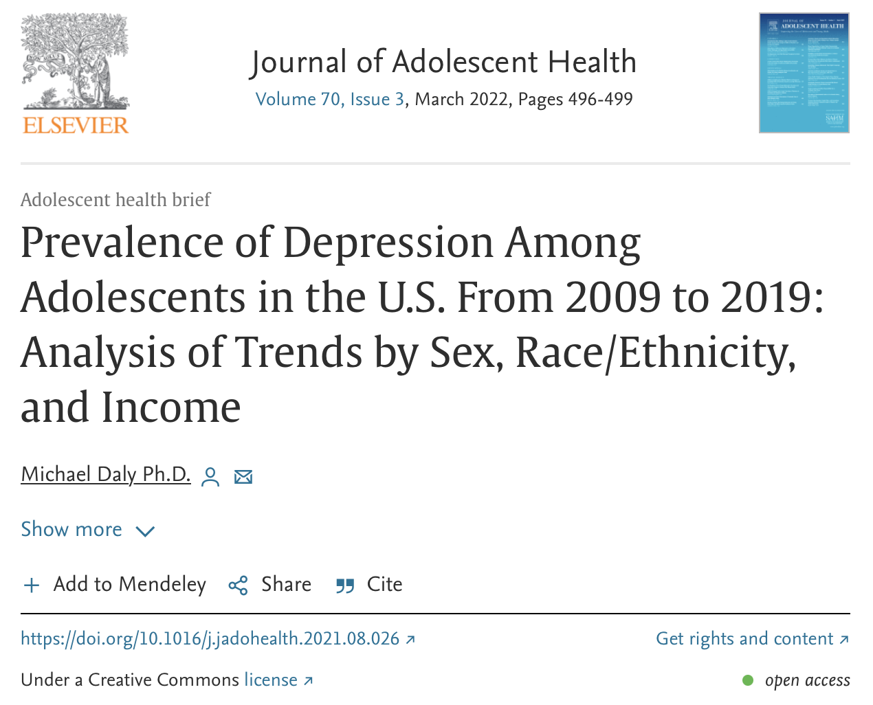
As described in the paper:
Depression is a leading cause of impairment and disability globally and major contributor to suicidal behavior. The prevalence of fatal suicide among U.S. adolescents and young adults increased by 57.4% between 2007 and 2018. This trend has been attributed to a range of potential causes including increased prevalence of anxiety and depressive disorders over this period. Of particular concern is a rise in the prevalence of major depression reported by U.S. adolescents since 2010. Although national trends in depression have been documented, reliable up-to-date estimates of trends among key subpopulations are needed. To address this gap, this study drew on nationally representative data to estimate temporal trends in the prevalence of past-year major depressive episode (MDE) across sex, race/ethnicity, and household income groups between 2009 and 2019.
We will take a look at the prevalence of Major Depressive Episodes (MDE) across sex from 2009 to 2019.
Before we begin, let’s load the libraries that we will need for the next tasks:
The data frame that we will use includes the following variables:
| Variable | Description |
|---|---|
| record_id | Unique ID for participant |
| year | Survey year |
| sex | Biological sex of respondent |
| age | Age of respondent |
| raceeth | Race/ethnicity of respondent |
| mde_past_year | Did the respondent meet criteria for a major depressive episode in the past-year? negative = did not meet criteria, positive = did meet criteria. |
| mde_lifetime | Did the respondent meet criteria for a major depressive episode in their lifetime? negative = did not meet criteria, positive = did meet criteria. |
| mh_sawprof | Did the respondent see a mental health care professional in the past-year? Response options include did not receive care, received care. |
| severity_chores | If mde_pastyear is positive, how severely did depression interfere with doing home chores? |
| severity_work | If mde_pastyear is positive, how severely did depression interfere with school/work? |
| severity_family | If mde_lifetime is positive, how severely did depression interfere with family relationships? |
| severity_chores | If mde_pastyear is positive, how severely did depression interfere with social life? |
| mde_lifetime_severe | If mde_pastyear is positive, was the MDE classified as severe? |
| substance_disorder | Did the respondent meet criteria for a past-year substance use disorder (alcohol or drug)? — available for 2019 data only — negative = did not meet criteria, positive = did meet criteria. |
| adol_weight | Sampling weight - from sampling protocol |
| vestr | Stratum — from sampling protocol |
| verep | Primary sampling unit — from sampling protocol |
This is a really large data frame, let’s import the whole data frame — and then print out the first 10 rows.
nsduh_20092019 <- read_rds(here("data", "NSDUH_adol_depression.Rds"))
nsduh_20092019 |> head(n = 10)
To gain a little more initial insight and familiarize ourselves with the data frame, here is a glimpse of the data frame.
nsduh_20092019 |> glimpse()Rows: 172,183
Columns: 17
$ record_id <chr> "2009_60065143", "2009_12006143", "2009_97316143",…
$ year <dbl> 2009, 2009, 2009, 2009, 2009, 2009, 2009, 2009, 20…
$ sex <chr> "male", "female", "male", "male", "male", "female"…
$ age <dbl> 14, 17, 16, 17, 12, 17, 15, 13, 15, 16, 12, 15, 15…
$ raceeth <chr> "Hispanic", "Black", "Non-hispanic White", "Non-hi…
$ mde_lifetime <chr> NA, "negative", "negative", "negative", "negative"…
$ mde_pastyear <chr> NA, "negative", "negative", "negative", "negative"…
$ mde_pastyear_severe <chr> NA, "negative", "negative", "negative", "negative"…
$ mh_sawprof <chr> NA, NA, NA, NA, NA, NA, NA, "did not receive care"…
$ severity_chores <dbl> NA, NA, NA, NA, NA, NA, NA, NA, NA, NA, NA, NA, NA…
$ severity_work <dbl> NA, NA, NA, NA, NA, NA, NA, NA, NA, NA, NA, NA, NA…
$ severity_family <dbl> NA, NA, NA, NA, NA, NA, NA, NA, NA, NA, NA, NA, NA…
$ severity_social <dbl> NA, NA, NA, NA, NA, NA, NA, NA, NA, NA, NA, NA, NA…
$ substance_disorder <chr> NA, NA, NA, NA, NA, NA, NA, NA, NA, NA, NA, NA, NA…
$ adol_weight <dbl> 3524.60777, 1951.52937, 881.28399, 284.11492, 632.…
$ vestr <dbl> 30017, 30012, 30019, 30017, 30027, 30058, 30031, 3…
$ verep <dbl> 1, 2, 1, 1, 1, 2, 1, 2, 1, 1, 1, 2, 1, 1, 1, 2, 2,…A skim of the data frame is also useful for getting familiar with the structure.
nsduh_20092019 |> skim()| Name | nsduh_20092019 |
| Number of rows | 172183 |
| Number of columns | 17 |
| _______________________ | |
| Column type frequency: | |
| character | 8 |
| numeric | 9 |
| ________________________ | |
| Group variables | None |
Variable type: character
| skim_variable | n_missing | complete_rate | min | max | empty | n_unique | whitespace |
|---|---|---|---|---|---|---|---|
| record_id | 0 | 1.00 | 13 | 13 | 0 | 172183 | 0 |
| sex | 0 | 1.00 | 4 | 6 | 0 | 2 | 0 |
| raceeth | 0 | 1.00 | 5 | 31 | 0 | 7 | 0 |
| mde_lifetime | 3731 | 0.98 | 8 | 8 | 0 | 2 | 0 |
| mde_pastyear | 4400 | 0.97 | 8 | 8 | 0 | 2 | 0 |
| mde_pastyear_severe | 4465 | 0.97 | 8 | 8 | 0 | 2 | 0 |
| mh_sawprof | 144086 | 0.16 | 13 | 20 | 0 | 2 | 0 |
| substance_disorder | 158786 | 0.08 | 8 | 8 | 0 | 2 | 0 |
Variable type: numeric
| skim_variable | n_missing | complete_rate | mean | sd | p0 | p25 | p50 | p75 | p100 | hist |
|---|---|---|---|---|---|---|---|---|---|---|
| year | 0 | 1.0 | 2013.60 | 3.15 | 2009.00 | 2011.00 | 2013.00 | 2016.00 | 2019.00 | ▇▅▃▅▃ |
| age | 0 | 1.0 | 14.56 | 1.69 | 12.00 | 13.00 | 15.00 | 16.00 | 17.00 | ▇▅▅▅▅ |
| severity_chores | 154761 | 0.1 | 5.54 | 2.39 | 1.00 | 4.00 | 6.00 | 7.00 | 10.00 | ▃▅▇▆▃ |
| severity_work | 154400 | 0.1 | 5.82 | 2.51 | 1.00 | 4.00 | 6.00 | 8.00 | 10.00 | ▃▅▇▇▅ |
| severity_family | 154264 | 0.1 | 6.29 | 2.53 | 1.00 | 5.00 | 6.00 | 8.00 | 10.00 | ▂▅▇▇▆ |
| severity_social | 154177 | 0.1 | 6.34 | 2.52 | 1.00 | 5.00 | 7.00 | 8.00 | 10.00 | ▂▅▇▇▇ |
| adol_weight | 0 | 1.0 | 1586.47 | 1425.59 | 1.04 | 571.59 | 1222.21 | 2150.64 | 22959.61 | ▇▁▁▁▁ |
| vestr | 0 | 1.0 | 34782.51 | 4991.52 | 30001.00 | 30029.00 | 30058.00 | 40024.00 | 40050.00 | ▇▁▁▁▇ |
| verep | 0 | 1.0 | 1.50 | 0.50 | 1.00 | 1.00 | 2.00 | 2.00 | 2.00 | ▇▁▁▁▇ |
Important
Please take a moment to read through these basic descriptions just presented to familiarize yourself with the data frame and variables within it.
Some Initial Computations
With some basic understanding of the data frame — let’s now dig in and describe the data more thoroughly. Notice from our summaries above that the data frame includes 172,183 adolescents. These adolescents were surveyed during one year sometime between 2009 and 2019. We can use the group_by() and tally() functions from the tidyverse to determine how many adolescents participated each year.
Calculate the number of participants at each wave
The functions group_by() and tally() serve to count and display the number of adolescents who took part in the survey each year.
nsduh_20092019 |>
  group_by(year) |>
  tally()
For example, we see that in 2009, 17,527 adolescents participated in the interview.
Calculate the number of male and female participants at each wave
What if we wanted to determine how many males and females participated each year? Simple — just add sex to the group_by() function code:
nsduh_20092019 |>
  group_by(year, sex) |>
  tally()
For example, here we see that in 2009, 8,650 participants reported being female and 8,877 reported being male.
Create a publication-ready table of participation
The group_by() and tally() functions are great for obtaining descriptive summaries as you comb through and conduct your analysis. But, you may want a table that is more publication-ready. The gtsummary package is an excellent resource for this endeavor. Let’s see how it can work for our present application. We’ll use the package’s tbl_summary() function here.
nsduh_20092019 |>
  select(year, sex) |>
tbl_summary(by = sex)| Characteristic | female N = 84,3771 |
male N = 87,8061 |
|---|---|---|
| year | 2,013.0 (2,011.0, 2,016.0) | 2,013.0 (2,011.0, 2,016.0) |
| 1 Median (Q1, Q3) | ||
In the code chunk, we selected our two variables of interest (year and sex), then we requested a summary table of this subsetted data frame, stratified by sex. The table relies just on the defaults of tbl_summary() — and the default for a numeric, continuous variable1 is to print the median and interquartile range (IQR). This isn’t terribly useful in this context. So, we need to add customization to get a more useful table. There are many options available to create a table that is right for your application. Here’s a new version of the table that adds customization.
nsduh_20092019 |>
  select(year, sex) |>
  tbl_summary(by = sex,
              type = list(year ~ "categorical"),
              label = year ~ "Year of Survey") |>
  as_gt() |>
tab_header(title = md("**Table 1. Number of participants by year and sex**"))| Table 1. Number of participants by year and sex | ||
|---|---|---|
| Characteristic | female N = 84,3771 |
male N = 87,8061 |
| Year of Survey | ||
| 2009 | 8,650 (10%) | 8,877 (10%) |
| 2010 | 9,049 (11%) | 9,345 (11%) |
| 2011 | 9,383 (11%) | 9,881 (11%) |
| 2012 | 8,613 (10%) | 8,786 (10%) |
| 2013 | 8,617 (10%) | 9,119 (10%) |
| 2014 | 6,690 (7.9%) | 6,910 (7.9%) |
| 2015 | 6,677 (7.9%) | 6,908 (7.9%) |
| 2016 | 6,984 (8.3%) | 7,288 (8.3%) |
| 2017 | 6,672 (7.9%) | 7,050 (8.0%) |
| 2018 | 6,501 (7.7%) | 6,786 (7.7%) |
| 2019 | 6,541 (7.8%) | 6,856 (7.8%) |
| 1 n (%) | ||
Here we see that for each year, tbl_summary() provides the number of adolescents who completed the survey as well as the percentage of the column. For example, in 2009, 8,650 females completed the survey — which is 10% of the females who completed the survey across the 11 years (2009 to 2019) - i.e., 8,650/84,377 = 10%).
Let’s break down the code to create this table step by step:
nsduh_20092019: This is the data frame and it is piped,|>, into the subsequent function.select(year, sex): The select() function is used to select two variables from the data frame, year and sex. This indicates that the subsequent analysis will only focus on these two variables — this is important here because relying on the defaults, tbl_summary() will create a table that includes all of the variables being fed into the function.tbl_summary(by = sex, type = list(year ~ "categorical"), label = year ~ "Year of Survey"): The tbl_summary() function comes from the gtsummary package. The function takes several arguments:by = sex: This argument indicates that the summary table should be stratified by the sex variable, meaning there will be separate summaries for each sex.type = list(year ~ "categorical"): This argument specifies that the year variable should be treated as a categorical variable in the summary table. When excluded (as you can see in the first version of the table), tbl_summary() treats this variable as a continuous variable and provides summary statistics (e.g., the median and interquartile range is the default for continuous, numeric variables).label = year ~ "Year of Survey": This argument renames the label of the year variable to “Year of Survey” in the summary table.
as_gt(): This converts the summarized table to a gt object. The gt package offers countless methods for further customization. Here, we use the tab_header() function from the package to add a title. The md() function, which is part of gt, renders text as Markdown2. In this context,md("**Table 1. Number of participants by year and sex**")converts the string into Markdown format, allowing for the use of Markdown syntax to style the text. Here, the double asterisks around the text make it bold. If interested, you can learn a lot more about Markdown here.
Explore the 2019 NSDUH Data
Before we dive into replicating the Daly paper mentioned above, and estimating the proportion of male and female adolescents who experienced a MDE in the past-year — let’s explore just the 2019 data a bit. We will begin by creating a version of the data frame that includes just year 2019.
nsduh_2019 <-
  nsduh_20092019 |>
  filter(year == 2019)
A table of all relevant variables
Using the 2019 data frame, let’s request a quick summary of all of the relevant variables in the data frame using the tbl_summary() function again. Notice that now, we select several variables to describe, but we do not stratify by sex. This will just give us basic information about the variables collected in 2019 as a whole.
nsduh_2019 |>
  select(sex, age, raceeth, starts_with("MDE"), starts_with("severity"), mh_sawprof, substance_disorder) |>
tbl_summary()| Characteristic | N = 13,3971 |
|---|---|
| sex | |
| female | 6,541 (49%) |
| male | 6,856 (51%) |
| age | |
| 12 | 2,086 (16%) |
| 13 | 2,247 (17%) |
| 14 | 2,222 (17%) |
| 15 | 2,323 (17%) |
| 16 | 2,293 (17%) |
| 17 | 2,226 (17%) |
| raceeth | |
| Asian | 550 (4.1%) |
| Black | 1,781 (13%) |
| Hispanic | 3,186 (24%) |
| Multiracial | 747 (5.6%) |
| Native American | 206 (1.5%) |
| Native Hawaiin/Pacific Islander | 64 (0.5%) |
| Non-hispanic White | 6,863 (51%) |
| mde_lifetime | |
| negative | 10,146 (78%) |
| positive | 2,869 (22%) |
| Unknown | 382 |
| mde_pastyear | |
| negative | 10,852 (84%) |
| positive | 2,098 (16%) |
| Unknown | 447 |
| mde_pastyear_severe | |
| negative | 11,439 (88%) |
| positive | 1,497 (12%) |
| Unknown | 461 |
| severity_chores | 6.00 (4.00, 7.00) |
| Unknown | 11,432 |
| severity_work | 6.00 (4.00, 8.00) |
| Unknown | 11,400 |
| severity_family | 6.00 (5.00, 8.00) |
| Unknown | 11,415 |
| severity_social | 7.00 (5.00, 8.00) |
| Unknown | 11,396 |
| mh_sawprof | |
| did not receive care | 1,777 (61%) |
| received care | 1,114 (39%) |
| Unknown | 10,506 |
| substance_disorder | |
| negative | 12,741 (95%) |
| positive | 656 (4.9%) |
| 1 n (%); Median (Q1, Q3) | |
Add variable labels to the table
This is a fine table, however, the variable names are recorded. Instead, a label that describes the variable would be preferred. We can do this in one of two ways. First, we can add labels directly to our tbl_summary() function. Here’s an example of this approach:
nsduh_2019 |>
  select(sex, age, raceeth, starts_with("MDE"), starts_with("severity"), mh_sawprof, substance_disorder) |>
  tbl_summary(label = list(
    sex ~ "Sex",
    age ~ "Age",
    raceeth ~ "Race/ethnicity",
    mde_lifetime ~ "Lifetime prevalence of a Major Depressive Episode",
    mde_pastyear ~ "Past-year prevalence of a Major Depressive Episode",
    mde_pastyear_severe ~ "Past-year prevalence of a severe Major Depressive Episode",
    severity_chores ~ "MDE-caused interference with doing home chores",
    severity_work ~ "MDE-caused interference with ability to function at school/work",
    severity_family ~ "MDE-caused interference with family relationships",
    severity_social ~ "MDE-caused interference with social life",
    mh_sawprof ~ "Saw a professional for mental health care in past-year",
    substance_disorder ~ "Past-year prevalence of a substance use disorder"
))| Characteristic | N = 13,3971 |
|---|---|
| Sex | |
| female | 6,541 (49%) |
| male | 6,856 (51%) |
| Age | |
| 12 | 2,086 (16%) |
| 13 | 2,247 (17%) |
| 14 | 2,222 (17%) |
| 15 | 2,323 (17%) |
| 16 | 2,293 (17%) |
| 17 | 2,226 (17%) |
| Race/ethnicity | |
| Asian | 550 (4.1%) |
| Black | 1,781 (13%) |
| Hispanic | 3,186 (24%) |
| Multiracial | 747 (5.6%) |
| Native American | 206 (1.5%) |
| Native Hawaiin/Pacific Islander | 64 (0.5%) |
| Non-hispanic White | 6,863 (51%) |
| Lifetime prevalence of a Major Depressive Episode | |
| negative | 10,146 (78%) |
| positive | 2,869 (22%) |
| Unknown | 382 |
| Past-year prevalence of a Major Depressive Episode | |
| negative | 10,852 (84%) |
| positive | 2,098 (16%) |
| Unknown | 447 |
| Past-year prevalence of a severe Major Depressive Episode | |
| negative | 11,439 (88%) |
| positive | 1,497 (12%) |
| Unknown | 461 |
| MDE-caused interference with doing home chores | 6.00 (4.00, 7.00) |
| Unknown | 11,432 |
| MDE-caused interference with ability to function at school/work | 6.00 (4.00, 8.00) |
| Unknown | 11,400 |
| MDE-caused interference with family relationships | 6.00 (5.00, 8.00) |
| Unknown | 11,415 |
| MDE-caused interference with social life | 7.00 (5.00, 8.00) |
| Unknown | 11,396 |
| Saw a professional for mental health care in past-year | |
| did not receive care | 1,777 (61%) |
| received care | 1,114 (39%) |
| Unknown | 10,506 |
| Past-year prevalence of a substance use disorder | |
| negative | 12,741 (95%) |
| positive | 656 (4.9%) |
| 1 n (%); Median (Q1, Q3) | |
Alternatively, we can add variable labels directly to the data frame — and then request the table. For this, we need the labelled package, specifically it’s set_variable_labels() function. Labelling all of your variables up front can save you time, because, once added, any time you use the data frame — the labels will be printed out.
To use the set_variable_labels() function, simply list the variable name, followed by = and the label you want to provide in quotations. Before applying labels to the full data frame — take a look at the simple example below to provide a label for year. The str() function gives details on the structure of an object — when I request this — you can see that year now has a label associated with it.
nsduh_2019 |>
  labelled::set_variable_labels(
    year = "Data collection year") |>
  select(year) |>
  str()
tibble [13,397 × 1] (S3: tbl_df/tbl/data.frame)
$ year: num [1:13397] 2019 2019 2019 2019 2019 ...
..- attr(*, "label")= chr "Data collection year"Now, let’s apply labels to all of the variables.
nsduh_2019 <-
nsduh_2019 |>
  labelled::set_variable_labels(
    record_id = "Participant ID",
    year = "Data collection year",
    sex = "Sex",
    age = "Age",
    raceeth = "Race/ethnicity",
    mde_lifetime = "Lifetime Major Depressive Episode",
    mde_pastyear = "Past-year Major Depressive Episode",
    mde_pastyear_severe = "Past-year severe Major Depressive Episode",
    severity_chores = "MDE-caused interference with doing home chores",
    severity_work = "MDE-caused interference with ability to function at school/work",
    severity_family = "MDE-caused interference with family relationships",
    severity_social = "MDE-caused interference with social life",
    mh_sawprof = "Saw a professional for mental health care in past-year",
    substance_disorder = "Past-year substance use disorder",
    adol_weight = "Sampling weight - from sampling protocol",
    vestr =  "Stratum --- from sampling protocol",
    verep = "Cluster replicates --- from sampling protocol")
Once the labels are formatted, we can use a nice function from the labelled package called look_for() — this function will create a handy data dictionary.
nsduh_2019 |>
  labelled::look_for() |>
  select(variable, label)
I’ll show you one last trick. I like the datatable() function from the DT package for printing the look_for() table because it’s searchable. Check out the output below.
nsduh_2019 |>
  labelled::look_for() |>
  select(variable, label) |>
  DT::datatable()
The searchable table above is nice to have in your analysis notebook because it provides a handy way for you (or a reader of your report) to search for variable names and their labels. This is particularly useful when you are reporting on a very large number of variables.
Moreover, because we added the variable labels directly to the data frame, when we use tbl_summary() to create a table, the variable labels from our data frame will be used. Let’s create the table one last time using the updated data frame with the labels. I will also add a title.
nsduh_2019 |>
  select(sex, age, raceeth, starts_with("MDE"), starts_with("severity"), mh_sawprof, substance_disorder) |>
  tbl_summary() |>
  as_gt() |>
  tab_header(
    title = md("**Table 2. Descriptive statistics for key variables**"),
    subtitle = "Data from the National Survey on Drug Use and Health, 2019"
)| Table 2. Descriptive statistics for key variables | |
|---|---|
| Data from the National Survey on Drug Use and Health, 2019 | |
| Characteristic | N = 13,3971 |
| Sex | |
| female | 6,541 (49%) |
| male | 6,856 (51%) |
| Age | |
| 12 | 2,086 (16%) |
| 13 | 2,247 (17%) |
| 14 | 2,222 (17%) |
| 15 | 2,323 (17%) |
| 16 | 2,293 (17%) |
| 17 | 2,226 (17%) |
| Race/ethnicity | |
| Asian | 550 (4.1%) |
| Black | 1,781 (13%) |
| Hispanic | 3,186 (24%) |
| Multiracial | 747 (5.6%) |
| Native American | 206 (1.5%) |
| Native Hawaiin/Pacific Islander | 64 (0.5%) |
| Non-hispanic White | 6,863 (51%) |
| Lifetime Major Depressive Episode | |
| negative | 10,146 (78%) |
| positive | 2,869 (22%) |
| Unknown | 382 |
| Past-year Major Depressive Episode | |
| negative | 10,852 (84%) |
| positive | 2,098 (16%) |
| Unknown | 447 |
| Past-year severe Major Depressive Episode | |
| negative | 11,439 (88%) |
| positive | 1,497 (12%) |
| Unknown | 461 |
| MDE-caused interference with doing home chores | 6.00 (4.00, 7.00) |
| Unknown | 11,432 |
| MDE-caused interference with ability to function at school/work | 6.00 (4.00, 8.00) |
| Unknown | 11,400 |
| MDE-caused interference with family relationships | 6.00 (5.00, 8.00) |
| Unknown | 11,415 |
| MDE-caused interference with social life | 7.00 (5.00, 8.00) |
| Unknown | 11,396 |
| Saw a professional for mental health care in past-year | |
| did not receive care | 1,777 (61%) |
| received care | 1,114 (39%) |
| Unknown | 10,506 |
| Past-year substance use disorder | |
| negative | 12,741 (95%) |
| positive | 656 (4.9%) |
| 1 n (%); Median (Q1, Q3) | |
Calculate the proportion of participants with MDE by sex
Using the 2019 data frame, let’s calculate the proportion of male and female participants who met the criteria for Major Depressive Episode (MDE) — we’ll obtain these proportions for both lifetime and past-year MDE.
nsduh_2019 |>
  select(mde_lifetime, mde_pastyear, sex) |>
  tbl_summary(by = sex) |>
  as_gt() |>
  tab_header(
    title = md("**Table 3. Prevalence of depression among U.S. adolescents by sex**"),
    subtitle = "Data from the National Survey on Drug Use and Health, 2019"
)| Table 3. Prevalence of depression among U.S. adolescents by sex | ||
|---|---|---|
| Data from the National Survey on Drug Use and Health, 2019 | ||
| Characteristic | female N = 6,5411 |
male N = 6,8561 |
| Lifetime Major Depressive Episode | ||
| negative | 4,352 (69%) | 5,794 (87%) |
| positive | 1,994 (31%) | 875 (13%) |
| Unknown | 195 | 187 |
| Past-year Major Depressive Episode | ||
| negative | 4,808 (76%) | 6,044 (91%) |
| positive | 1,487 (24%) | 611 (9.2%) |
| Unknown | 246 | 201 |
| 1 n (%) | ||
Important
Study the table to determine what proportion of males and females experienced a past-year MDE.
Calculate the proportion who received mental health care by sex
Perhaps we’d like to examine the prevalence of mental health care by sex among those with a past-year MDE. We can do that with the following code:
nsduh_2019 |>
  filter(mde_pastyear == "positive") |>
  select(mh_sawprof, sex) |>
  tbl_summary(by = sex) |>
  as_gt() |>
  tab_header(
    title = md("**Table 4. Prevalence of mental health care among adolescents with a past-year MDE**"),
    subtitle = "Data from the National Survey on Drug Use and Health, 2019"
)| Table 4. Prevalence of mental health care among adolescents with a past-year MDE | ||
|---|---|---|
| Data from the National Survey on Drug Use and Health, 2019 | ||
| Characteristic | female N = 1,4871 |
male N = 6111 |
| Saw a professional for mental health care in past-year | ||
| did not receive care | 812 (55%) | 378 (62%) |
| received care | 667 (45%) | 229 (38%) |
| Unknown | 8 | 4 |
| 1 n (%) | ||
Examine severity of depression items
Building on the last example, let’s take a look at information about the severity of depression. To measure this construct (i.e., severity of depression) the level of functional impairment caused by poor mental health over the course of the past 12 months was assessed using the Sheehan Disability Scale (SDS).
For adolescents, the SDS measures mental health-related impairment in four major life activities or role domains:
Chores at home
Ability to do well at school or work
Ability to get along with family
Ability to have a social life
For adolescents with a past-year MDE, respondents were instructed to think about the time in the past 12 months when problems with their mood were at their worst and use the 0 to 10 scale to describe how much their depression symptoms caused problems in these four areas.
nsduh_2019 |>
  filter(mde_pastyear == "positive") |>
  select(starts_with("severity_"), sex) |>
  tbl_summary(by = sex,
                         statistic = list(starts_with("severity_") ~ "{mean} ({sd})"),
                         missing = "no") |>
  as_gt() |>
  tab_header(
    title = md("**Table 5. Impacts of depression among adolescents with a past-year MDE**"),
    subtitle = "Data from the National Survey on Drug Use and Health, 2019"
)| Table 5. Impacts of depression among adolescents with a past-year MDE | ||
|---|---|---|
| Data from the National Survey on Drug Use and Health, 2019 | ||
| Characteristic | female N = 1,4871 |
male N = 6111 |
| MDE-caused interference with doing home chores | 5.62 (2.36) | 5.59 (2.29) |
| MDE-caused interference with ability to function at school/work | 5.88 (2.57) | 5.90 (2.54) |
| MDE-caused interference with family relationships | 6.36 (2.45) | 5.84 (2.52) |
| MDE-caused interference with social life | 6.48 (2.51) | 6.10 (2.56) |
| 1 Mean (SD) | ||
There are a couple of new options for tbl_summary() that I used in this chunk of code. First, notice that I used the statistic = argument to specify that, for the severity variables, the mean and the standard deviation (in parentheses) should be printed. Recall that the default for a numeric continuous variable is the median and IQR. I also used the missing = "no" argument to suppress printing the missing/unknown cases (which declutters the table).
Use graphs to display the individual severity items
The table we just created is informative, but we can further explore these severity variables with a plot. Let’s create both a histogram and a density plot to display the distribution of each severity score for males and females. First though, because we want to facet the plots by the severity item (e.g., chores, school, family, social) we need to pivot the data to longer using the pivot_longer() function (which we learned about in Module 04). In this pivoted data frame — each adolescent will have up to 4 rows of data — one for each of the severity items that they reported on.
First, let’s pivot the data.
severity_long <-
nsduh_2019 |>
  filter(mde_pastyear == "positive") |>
  select(record_id, sex, starts_with("severity_")) |>
  pivot_longer(cols = starts_with("severity_"), names_to = "variable", values_to = "score") |>
  drop_na()

severity_long |>
  head(n = 20)
Now, we can create the plots. First, here is the histogram.
severity_long |>
  ggplot(mapping = aes(x = score, fill = sex)) +
    geom_histogram(binwidth = 1) +
    facet_wrap(~ variable) +
    theme_minimal() +
  labs(title = "Histogram of MDE-caused severity items for males and females",
       x = "Severity Score")
Now, here is the density plot.
# Density plot
severity_long |>
  ggplot(mapping = aes(x = score, fill = sex)) +
    geom_density(alpha = 0.5) +
    facet_wrap(~ variable) +
    theme_minimal() +
  labs(title = "Density plot of MDE-caused severity items for males and females",
       x = "Severity Score")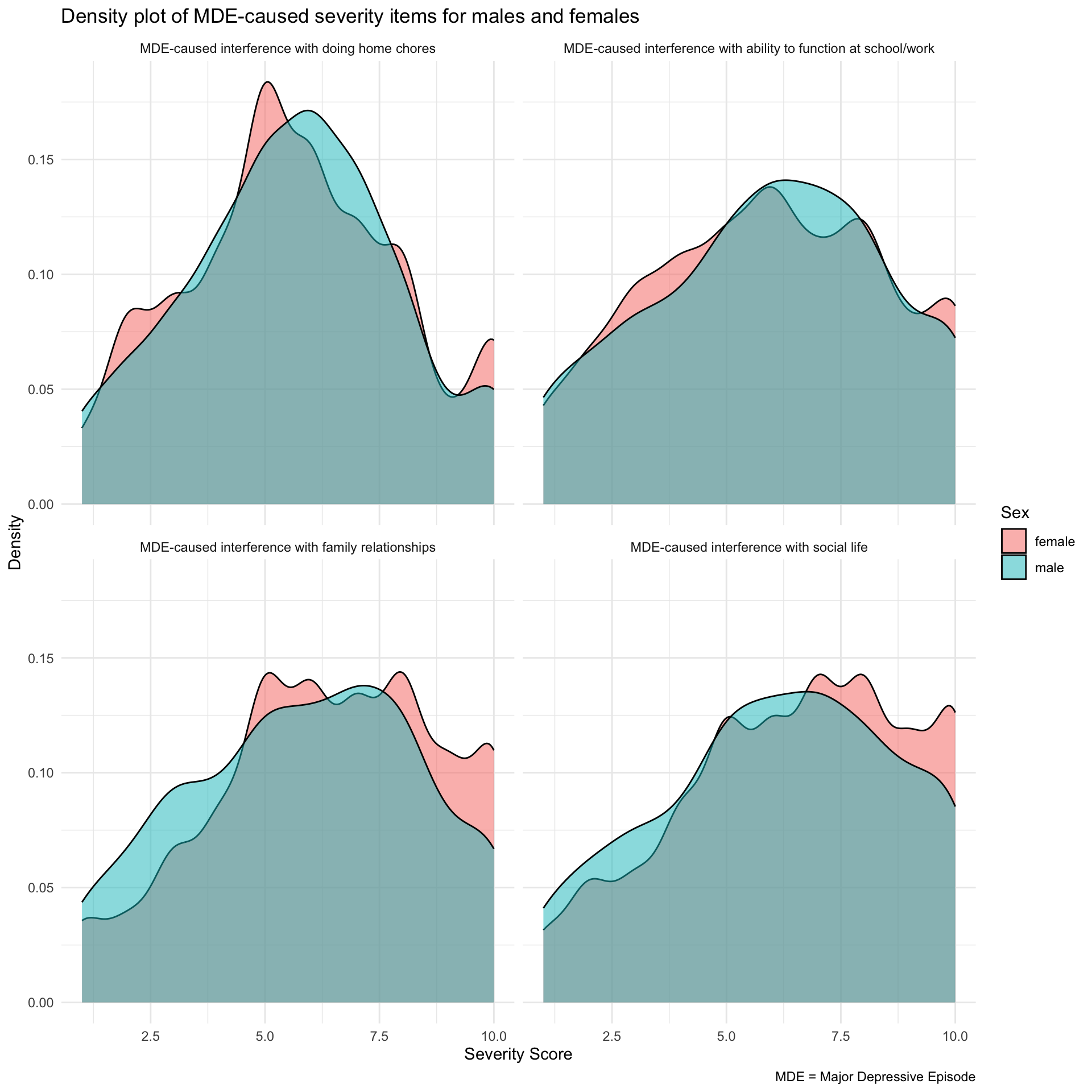
In the histogram, you’ll notice that the bars for females are considerably higher than those for males. This is because the histogram reflects not only the distribution but also the number of cases — in this instance, 24% of females compared to about 9% of males met the criteria for MDE and reported on these symptom severity items. That is, in the histogram, the height of the bars represents the number of cases (or frequency) within each score range. The higher frequency for females is visually evident in the taller bars. Thus, because histograms show raw counts, they help us understand not only the distribution but also the number of observations in each category.
On the other hand, the density plots appear similar for males and females. Density plots focus on the shape of the distribution rather than the actual counts. They provide a smoothed version of the histogram and are normalized so that the area under the curve sums to 1. This normalization means that the density plot for males and females can appear similar, even if the actual number of cases is different. The density plot allows us to compare the distribution shapes of severity scores between males and females without being influenced by the different sample sizes.
Both the histograms and density plots have benefits and drawbacks, and these are apparent in the examples we created.
Histograms are excellent for visually capturing the difference in the number of cases between two groups, making the disparity in prevalence immediately apparent. However, the variation in counts can overshadow the underlying distribution of the data.
Density plots, on the other hand, are useful for comparing the shapes of distributions without getting distracted by the difference in sample sizes. However, they do not portray the actual prevalence in the sample.
Refine the density graph
Let’s assume we prefer the density plot and want to improve its readability. Notice that the facets in the previous graph currently display variable names, which may not clearly communicate their meaning to the reader. To enhance interpretability, we can assign more descriptive labels to these facets. A straightforward approach to accomplish this in R involves converting the facet variable into a factor with clearly defined, descriptive labels.
In R, factors are used to represent categorical data — variables with a fixed set of unique values (or levels), such as gender or treatment groups. Factors are especially useful for statistical modeling and data visualization because they enable R to properly handle categorical information. Additionally, factors allow you to assign clear, descriptive labels to each category, making your results more interpretable.
The factor() function in R converts a variable into a factor, a special type of vector designed for categorical data. It assigns each unique value a specific level and allows you to provide descriptive labels for those levels. In the example below, the factor() function is used to clearly label each severity variable, enhancing interpretability and preparing the data for improved visualization. The levels = argument specifies the original column names, while the labels = argument provides descriptive labels for these levels. The ordering of the levels and labels should be consistent, so, for example, severity_chores (the first level listed) corresponds to MDE-caused interference with doing home chores (the first label listed).
Notice that in the newly created graph, an informative label, rather than the variable name, denotes each facet.
severity_long <-
nsduh_2019 |>
  filter(mde_pastyear == "positive") |>
  select(record_id, sex, starts_with("severity_")) |>
  pivot_longer(cols = starts_with("severity_"), names_to = "variable", values_to = "score") |>
  drop_na() |>
  mutate(variable = factor(variable,
                           levels = c("severity_chores", "severity_work", "severity_family", "severity_social"),
                           labels = c("MDE-caused interference with doing home chores",
                                      "MDE-caused interference with ability to function at school/work",
                                      "MDE-caused interference with family relationships",
                                      "MDE-caused interference with social life")))


severity_long |>
  ggplot(mapping = aes(x = score, fill = sex)) +
    geom_density(alpha = 0.5) +
    facet_wrap(~ variable) +
    theme_minimal() +
  labs(title = "Density plot of MDE-caused severity items for males and females",
       x = "Severity Score",
       y = "Density",
       fill = "Sex",
       caption = "MDE = Major Depressive Episode")
Create a variable that combines the severity items into one scale
Instead of considering each severity item separately, we might have an interest in combining them to form a composite score. One common method for this is to take the average of the items. Let’s form a severity scale that takes the average of the 4 severity items. This article shows a variety of ways to perform row-wise operations (i.e., averaging or summing across rows of your data frame) — I’ll demonstrate a straightforward way to accomplish this below using two helpful functions: rowMeans() and pick().
nsduh_2019_scale <-
nsduh_2019 |>
  filter(mde_pastyear == "positive") |>
  select(sex, starts_with("severity_")) |>
  mutate(severity_scale = rowMeans(pick(severity_chores, severity_work, severity_family, severity_social)))

nsduh_2019_scale |> select(starts_with("severity_")) |> head()
Here’s a breakdown of the code to create the scale score:
pick(severity_chores, severity_work, severity_family, severity_social): This expression uses the pick() function from the tidyverse to select certain variables from the existing data — i.e., the severity items.rowMeans(...): This function calculates the mean value of each row (i.e. for each adolescent). This will return a single value for each row in the data frame, representing the mean of the selected variables for that row.mutate(severity_scale = ...): This adds a new column to the data. The new column/variable will be named severity_scale, and its values will be the row-wise means calculated by rowMeans().
In summary, this code chunk calculates an average severity score across the four selected variables for each adolescent in the data frame.
If you’ve been careful and deliberate with naming the variables that will go into your scale, you can use a short cut that saves you from typing each variable name — check out the use of starts_with() in the code below:
nsduh_2019_scale <-
nsduh_2019 |>
  filter(mde_pastyear == "positive") |>
  select(sex, starts_with("severity_")) |>
  mutate(severity_scale = rowMeans(pick(starts_with("severity_"))))

nsduh_2019_scale |> select(starts_with("severity_")) |> head()
Notice that, by default, anyone who is missing one or more of the severity items will be assigned NA for the new scale score. This is because the default for rowMeans() is to drop cases with missing data. If instead you desired to form the mean with whatever variables were present, you could add na.rm = TRUE to the rowMeans() call as follows:
nsduh_2019_scale <-
nsduh_2019 |>
  filter(mde_pastyear == "positive") |>
  select(sex, starts_with("severity_")) |>
  mutate(severity_scale = rowMeans(pick(starts_with("severity_")), na.rm = TRUE))

nsduh_2019_scale |> select(starts_with("severity_")) |> head()
Alternatively, with a little more coding you could specify that you’d like the scale to be formed only if a certain number of the items are observed for the individual — for example, the code below requires that an individual answered at least 3 of the 4 severity items in order for the scale to be formed. This is a slightly more advanced specification that utilizes case_when() from Module 04.
nsduh_2019_scale <-
nsduh_2019 |>
  filter(mde_pastyear == "positive") |>
  select(sex, starts_with("severity_")) |>
  mutate(severity_scale = case_when(rowSums(!is.na(pick(starts_with("severity_")))) >= 3 ~ rowMeans(pick(starts_with("severity_")), na.rm = TRUE)))

nsduh_2019_scale |> select(starts_with("severity_")) |> head()
Use a graph to display the severity scale scores
We did all the work to form this new severity scale score — let’s take a moment to create a graph of the distribution of it across males and females. I’ll add a few extra options below to make it more attractive, including choosing different colors for sex and using patchwork to create side by side graphs of the histogram and density plot (click here for more information about these patchwork options).
group.colors <- c("male" = "#6ce1ff", "female" = "#e0ce75")

hist <-
nsduh_2019_scale |>
  drop_na() |>
  ggplot(mapping = aes(x = severity_scale, fill = sex)) +
  geom_histogram(binwidth = 0.5) +
  scale_fill_manual(values = group.colors) +
  theme_minimal() +
  theme(legend.position = "none") +
  labs(title = "A histogram of the data",
       x = "Severity of MDE",
       y = "Count",
       fill = "Biological Sex")

dens <-
nsduh_2019_scale |>
  drop_na() |>
  ggplot(mapping = aes(x = severity_scale, fill = sex)) +
  geom_density(alpha = 0.75) +
  scale_fill_manual(values = group.colors) +
  theme_minimal() +
  labs(title = "A density plot of the data",
       x = "Severity of MDE",
       y = "Density",
       fill = "Sex")


library(patchwork)

my_plots <- hist + dens
my_plots + plot_annotation(
  title = "Distribution of the MDE severity score among adolescents with a past-year MDE",
  subtitle = "Data from the National Survey on Drug Use and Health (NSDUH), 2019",
  caption = "MDE = Major Depressive Episode; 24% of adoelscent females and 9.2% of adolescent males in the 2019 NSDUH survey met criteria for a past-year MDE."
)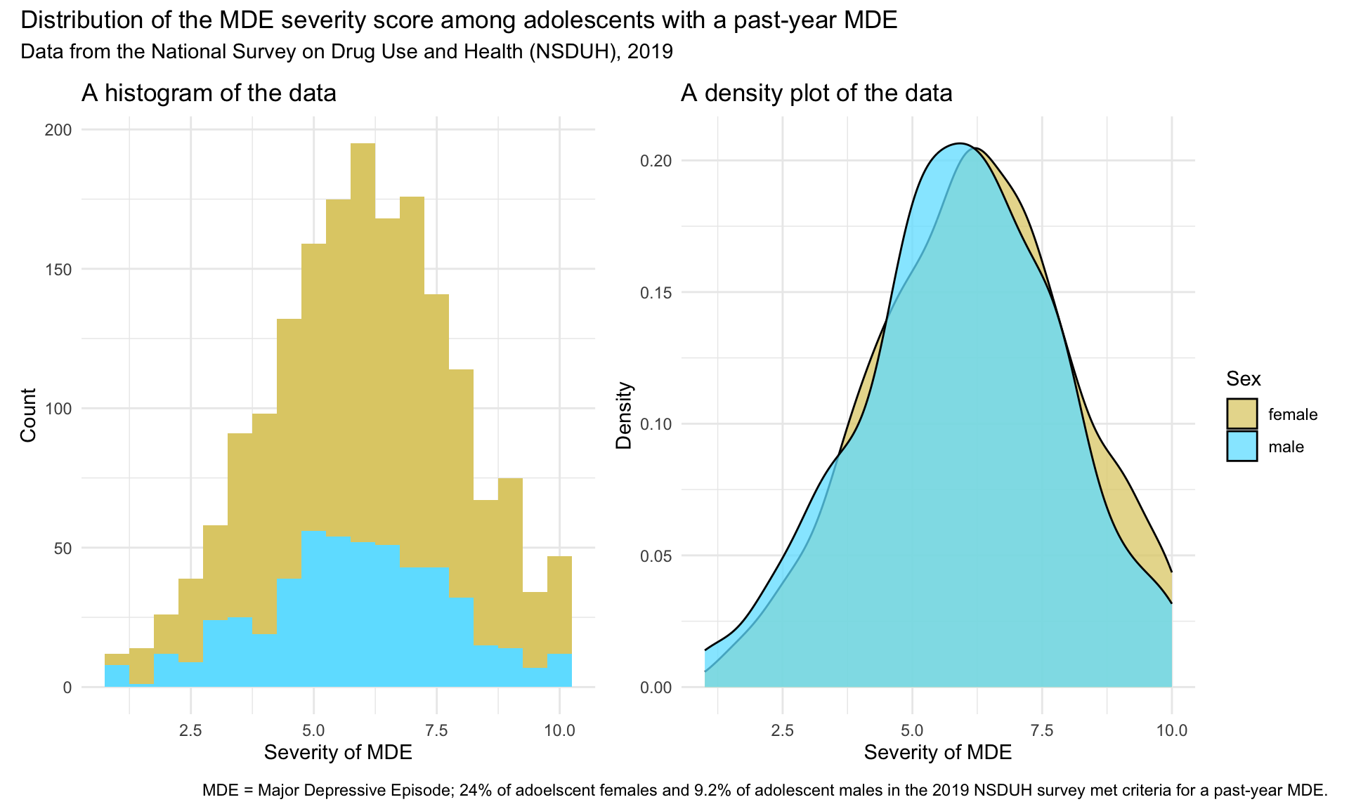
Looks great! Which graph do you prefer — the histogram or the density plot?
Cross tabulations of categorical/qualitative data
Cross tabulation of MDE and substance use disorder
Before returning to the full data frame (with all years between 2009 and 2019), let’s explore methods for looking at a cross tabulation of variables. We explored cross tabulations a bit in Module 05, where we learned about and practiced using the tbl_cross() function from the gtsummary package to obtain a cross tabulation of two categorical variables. Recall that a cross tabulation is a statistical tool used for analyzing the relationship between two or more categorical variables. It’s a type of table that displays the frequency distribution of the variables in a matrix format, making it easier to understand the relationship between them.
In a basic cross-tabulation with two variables, rows usually represent categories of one variable and columns represent categories of another variable. The cells in the table contain the counts or frequencies of the combined categories.
Let’s examine the relationship between past-year MDE (mde_pastyear) and past-year substance use disorder (substance_disorder) using a cross tabulation.
nsduh_2019 |>
  select(mde_pastyear, substance_disorder) |>
  tbl_cross(row = mde_pastyear, col = substance_disorder)
Past-year substance use disorder
|
Total | ||
|---|---|---|---|
| negative | positive | ||
| Past-year Major Depressive Episode | |||
| negative | 10,460 | 392 | 10,852 |
| positive | 1,856 | 242 | 2,098 |
| Unknown | 425 | 22 | 447 |
| Total | 12,741 | 656 | 13,397 |
In the table above, past-year MDE is displayed on the rows, and past-year substance disorder is displayed on the columns. We can switch these if we like (i.e, switch the variables listed in the row = and col = arguments).
Let’s explore some additional useful options to enhance our table. We can request percentages in addition to counts.
Row percent
First, let’s request percents to be calculated by row (i.e., past-year MDE in our example). Notice the argument percent = "row" in the code below. With this option, each row will sum to 100%, allowing us to compare the distribution of the column variable within each level of the row variable.
Notice also in the code below that after selecting the desired variables, I include drop_na(). This drops all missing data in a list-wise fashion — so any individuals with missing data on either variable in the cross-tabulation will be removed before computing and displaying the cross table.
nsduh_2019 |>
  select(mde_pastyear, substance_disorder) |>
  drop_na() |>
  tbl_cross(row = mde_pastyear, col = substance_disorder, percent = "row")
Past-year substance use disorder
|
Total | ||
|---|---|---|---|
| negative | positive | ||
| Past-year Major Depressive Episode | |||
| negative | 10,460 (96%) | 392 (3.6%) | 10,852 (100%) |
| positive | 1,856 (88%) | 242 (12%) | 2,098 (100%) |
| Total | 12,316 (95%) | 634 (4.9%) | 12,950 (100%) |
The table shows us that there are a total of 2,098 adolescents who reported a past-year MDE, 242 of whom had a past-year substance disorder. This means that 12% (242/2098) of the adolescents who reported a past-year MDE, also reported a past-year substance use disorder. On the other hand, there are a total of 10,852 adolescents who did not report a past-year MDE in the sample, and 392 (representing 3.6% of the sample of adolescents without a past-year MDE, that is 392/10852) had a substance use disorder. Summarizing this information, the prevalence of a past-year substance use disorder is much more common (about three times more common) among adolescents with a past-year MDE than adolescents without a past-year MDE.
Column percent
How does the table change if we specify percent = "column" instead of percent = "row"? With this option, each column will sum to 100%, allowing us to compare the distribution of the row variable within each level of the column variable.
nsduh_2019 |>
  select(mde_pastyear, substance_disorder) |>
  drop_na() |>
  tbl_cross(row = mde_pastyear, col = substance_disorder, percent = "column")
Past-year substance use disorder
|
Total | ||
|---|---|---|---|
| negative | positive | ||
| Past-year Major Depressive Episode | |||
| negative | 10,460 (85%) | 392 (62%) | 10,852 (84%) |
| positive | 1,856 (15%) | 242 (38%) | 2,098 (16%) |
| Total | 12,316 (100%) | 634 (100%) | 12,950 (100%) |
With the percents displayed relative to the columns, we find that there are a total of 634 adolescents who had a substance use disorder in the past-year, 38% (242/634) of those adolescents had a past-year MDE, and 62% (392/634) did not have a past-year MDE. Likewise, a total of 12,316 adolescents did not have a substance use disorder, 15% of these adolescents reported a past-year MDE, and 85% did not report a past-year MDE.
Cell percent
There is one other option for displaying percentages that we can choose. The argument percent = "cell" provides the percentage of people in each cell relative to the overall total. That is, when percent = "cell" is used, each cell displays the percentage of the entire sample that falls into that specific category combination. All percentages sum to 100% across the full table.
nsduh_2019 |>
  select(mde_pastyear, substance_disorder) |>
  drop_na() |>
  tbl_cross(row = mde_pastyear, col = substance_disorder, percent = "cell")
Past-year substance use disorder
|
Total | ||
|---|---|---|---|
| negative | positive | ||
| Past-year Major Depressive Episode | |||
| negative | 10,460 (81%) | 392 (3.0%) | 10,852 (84%) |
| positive | 1,856 (14%) | 242 (1.9%) | 2,098 (16%) |
| Total | 12,316 (95%) | 634 (4.9%) | 12,950 (100%) |
In this table, the percent in each cell with respect to the grand total is displayed. For example, there are 242 adolescents who reported both a MDE and a substance use disorder in the past year, which equals 1.9% of the total sample (i.e., 242/12950). These adolescents could be classified as having co-morbidity with respect to depression and substance use issues — comorbidity is defined as having two or more illnesses or disorders occurring at the same time.
Replication of Daly Paper
Past-year MDE by sex from 2009 - 2019
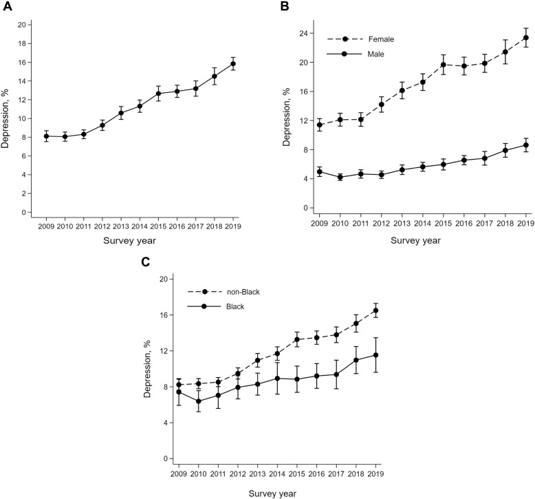
Now, let’s return to the full data frame that includes survey years between 2009 and 2019. This full data frame is what was used in the Daly (2021) paper described earlier. In this final section of the Module, we’ll reproduce panel B from this figure in the paper:
Let’s begin by subsetting the data frame to exclude cases missing on past-year MDE or sex.
for_trend_graph <-
  nsduh_20092019 |>
  select(year, sex, mde_pastyear) |>
  drop_na()
Now, let’s compute the proportion of males and females who met criteria for a past-year MDE in each survey year. Because mde_pastyear is a character variable — and we can’t calculate a proportion using a character variable, we need to first create a numeric variable so that we can perform our calculation. Here, the new variable is called mde_pastyear_positive and this new variable is coded 1 if the individual met the criteria for past-year MDE (i.e., mde_pastyear is equal to “positive”) and 0 if they did not meet criteria for a past-year MDE (i.e., mde_pastyear is equal to “negative”).
Once this variable is created we can group the data frame by year and sex, then compute the proportion. By calculating the mean of a binary variable coded 1 and 0 — the result is the proportion of cases coded 1 — which in our example indicates the proportion of individuals with a past-year MDE.
for_trend_graph_summary <-
  for_trend_graph|>
  mutate(mde_pastyear_positive = case_when(mde_pastyear == "positive"  ~ 1,
                                         mde_pastyear == "negative" ~ 0)) |>
  group_by(year, sex) |>
  summarize(proportion_mde_pastyear_positive = mean(mde_pastyear_positive, na.rm = TRUE), .groups = "drop")

for_trend_graph_summary
With this summarized data frame in hand, we can create our line graph. We’ll put year on the x-axis, and proportion_mde_pastyear_positive on the y-axis. We’ll also include the individual data points for each year to match the JAH graph we are replicating (via the geom_point() geometry). We’ll color the points and lines with the same colors we set earlier.
group.colors <- c("male" = "#6ce1ff", "female" = "#e0ce75")

for_trend_graph_summary |>
  ggplot(mapping = aes(x = year, y = proportion_mde_pastyear_positive, group = sex, color = sex)) +
  geom_line(linewidth = 2) +
  geom_point(size = 3) +
  scale_x_continuous(breaks = 2009:2019) +
  scale_y_continuous(limits = c(0,.25), labels = scales::percent_format(accuracy = 1)) +
  theme_minimal() +
  scale_color_manual(values = group.colors) +
  labs(title = "Proportion of adolescents who met criteria for a past-year Major Depressive Episode (MDE)",
       subtitle = "Data from the National Survey on Drug Use and Health (NSDUH), 2009 - 2019",
       x = "Year",
       y = "Percent of adolescents meeting criteria for past-year MDE",
       color = "Sex")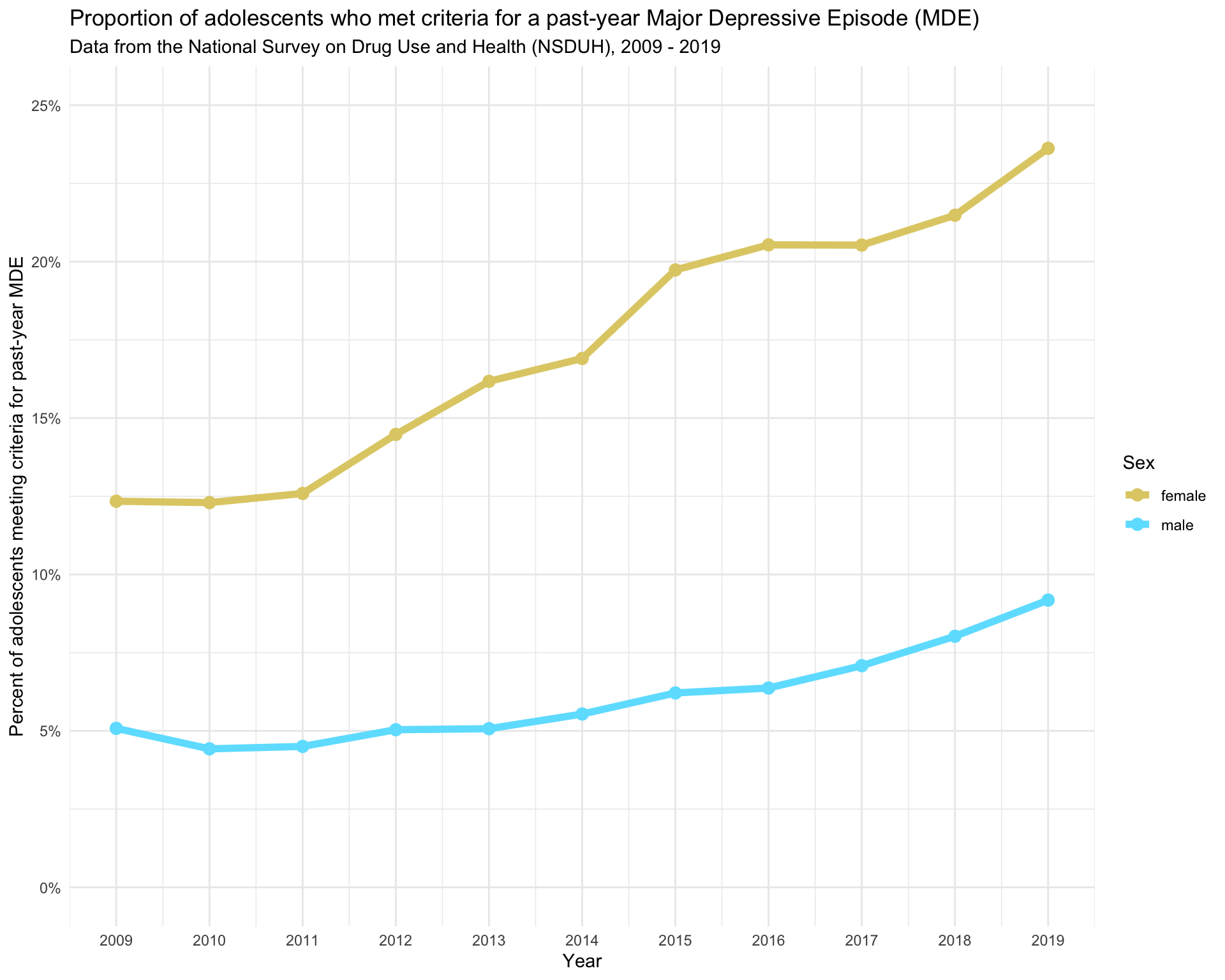
Our graph replicates the corresponding graph from the Daly (2021) paper. Note that the figure presented in the paper includes confidence intervals around the points. The confidence intervals denote the degree of uncertainty in the estimates. We’ll learn about confidence intervals and how to compute them in Module 08.
The Daly (2021) paper explains these findings as follows:
Depression levels among female participants increased by 12 percentage points (95% CI 10.4-13.5) between 2009 and 2019, from 11.4% to 23.4%. This increase was 8.3 percentage points (95% CI 6.2-10.4) larger than the increase experienced by males over the same period (3.7%, 95% CI 2.5-4.8) (Figure 1B). The gender difference in adolescent depression levels increased from 6.4 percentage points (95% CI 5.4-7.5) in 2009 to 14.8 percentage points (95% CI 12.9-16.6) in 2019.
And, includes the following discussion of the findings:
This study of over 160,000 adolescents aged 12-17 years drew on nationally representative data to show that the prevalence of MDE approximately doubled between 2009 and 2019 (from 8.1% to 15.8%). This prolonged rise in MDE is concerning because adolescent depression tends to persist into adulthood and forecasts adverse health and socioeconomic consequences throughout life.
In the current study, the gender disparity in depression more than doubled (from 6.4 to 14.8 percentage points) between 2009 and 2019 driven by a substantial rise in the prevalence of MDE among females over this period. This finding extends existing evidence that has found significant though less pronounced increases in internalizing problems and depressive symptoms among adolescent girls since the beginning of the 21st century. Potential reasons for this increase are manifold and include increases in bullying and victimization and use of social media and technology which may have been more impactful for girls than boys. In addition, reduced sleep quality and quantityy, the long-term impact of the Great Recession, and rising educational expectations may have contributed to the rise in depression.
Importantly, Daly (2021) also recognizes limitations of his study and findings:
The current study is limited in its reliance on self-reports of depressive symptoms that may differ from clinical evaluations and could be subject to recall bias. This study utilized repeated cross-sectional data and it remains possible that the surveyed populations differed over time, though the NSDUH’s high response rate, consistent sampling design, and use of survey weights safeguards against this possibility.
Last, the Daly (2021) paper offers these concluding remarks:
The results highlight the need for further investment in adolescent mental health promotion, mental health services, and intervention programs. School group-based interventions, exercise, and psychological therapy have demonstrated effectiveness in reducing adolescent depressive symptoms and could help tackle the marked rise in depression among adolescent girls identified in this study.
This brief documentary put together by the New York Times offers interesting insights into this ongoing crisis of adolescent depression.
Bonus Material: Getting Better Population Estimates
The NSDUH uses a stratified, multistage area probability sampling strategy to select participants, enabling it to produce nationally and state‑level representative estimates for the U.S. civilian, non‑institutionalized population aged 12 and older. This complex sampling is beyond the scope of this Module. For those interested, this resource gives an overview of the methodology.
For students interested in seeing how to adjust for the sampling strategy in R, I will provide the code below that can be used to obtain estimates of past-year and lifetime MDE for 2019 (i.e., Table 3 that we created earlier) that take into account the sampling design strategy. This uses the svydesign() function from the survey package, and the sampling variables described in the list of variables in the data frame (at the beginning of the Module).
First, here is a bit more information about the key sampling variables used in the NSDUH:
vestr: This variable identifies the sampling stratum. Stratification is used in survey sampling to divide the population into subgroups (strata) that share similar characteristics — often based on geography or demographics. Stratification helps ensure better representation of key subpopulations and improves the precision of survey estimates. Each stratum contains units that are relatively homogeneous with respect to characteristics important for the study.
verep: This variable identifies the Primary Sampling Unit (PSU). In the NSDUH’s multistage sampling design, PSUs are typically geographic areas (e.g., counties or groups of counties) selected in the first stage of sampling. Within each PSU, smaller units such as households or individuals are then sampled. Accounting for PSUs in the analysis is important for correctly estimating standard errors.
adol_weight: This is the final analysis weight for each adolescent respondent. It adjusts for the complex sampling design, including unequal probabilities of selection, nonresponse, and post-stratification to known population totals. Applying these weights ensures that the results are nationally representative. For example, if a respondent has a weight of 2, they represent two individuals in the broader U.S. adolescent population. These weights must be applied when estimating population-level proportions, means, or totals to ensure valid inferences.
So in summary, vestr, verep, and adol_weight are all variables in the NSDUH that play key roles in ensuring that the survey data is accurately representative of the larger population, allowing researchers to draw meaningful and valid conclusions about substance use and mental health in the United States.
And, here is the code that can be applied to obtain accurate population-level estimates for Table 3 that we estimated earlier for the 2019 data.
library(survey)

df_for_weighted <-
nsduh_2019 |>
  select(starts_with("mde_"), sex, adol_weight, vestr, verep)

weighted <-
  svydesign(
    id = ~ verep,
        strata = ~ vestr,
        data = df_for_weighted,
        weights = ~ adol_weight,
        nest = TRUE
    )

weighted |>
  tbl_svysummary(by = sex,
                            include = c("mde_lifetime", "mde_pastyear"),
                            label = list(
                              mde_lifetime ~ "Lifetime prevalence of a Major Depressive Episode",
                              mde_pastyear ~ "Past-year prevalence of a Major Depressive Episode")) |>
  as_gt() |>
  tab_header(
    title = md("**Table 3 (revised). Prevalence of depression among U.S. adolescents by sex**"),
    subtitle = "Data from the National Survey on Drug Use and Health, 2019") |>
   tab_footnote(
    footnote = "Table prevalences are adjusted for the NSDUH complex sample design",
    locations = cells_title(groups = "title")
)| Table 3 (revised). Prevalence of depression among U.S. adolescents by sex1 | ||
|---|---|---|
| Data from the National Survey on Drug Use and Health, 2019 | ||
| Characteristic | female N = 12,222,9892 |
male N = 12,682,0502 |
| Lifetime prevalence of a Major Depressive Episode | ||
| negative | 8,130,293 (69%) | 10,776,797 (87%) |
| positive | 3,728,867 (31%) | 1,556,756 (13%) |
| Unknown | 363,829 | 348,497 |
| Past-year prevalence of a Major Depressive Episode | ||
| negative | 9,019,046 (77%) | 11,252,466 (91%) |
| positive | 2,752,836 (23%) | 1,062,285 (8.6%) |
| Unknown | 451,107 | 367,298 |
| 1 Table prevalences are adjusted for the NSDUH complex sample design | ||
| 2 n (%) | ||
As you can see, the percentages are quite similar to our original Table 3 (which used the raw data) — but now we take into account the sampling design and the survey weights. The counts of people overall and in each cell are weighted to match the US population in 2019.
Account for survey design for Daly replication
As another example, we can compute better estimates for the replication of the Daly paper (i.e., estimates for the proportion of adolescents with a past-year MDE by year and sex) by taking into account the survey design. Here’s the code to carry out that process:
df_for_weighted_20092019 <-
  nsduh_20092019 |>
  select(year, starts_with("mde_"), sex, adol_weight, vestr, verep) |>
  mutate(mde_pastyear_positive = case_when(mde_pastyear == "positive"  ~ 1,
                                         mde_pastyear == "negative" ~ 0))

weighted_20092019 <-
  svydesign(
    id = ~ verep,
        strata = ~ vestr,
        data = df_for_weighted_20092019,
        weights = ~ adol_weight,
        nest = TRUE
    )

weighted_summary_20092019 <-
  svyby(
    formula = ~mde_pastyear_positive,
    by = ~year + sex,
    design = weighted_20092019,
    FUN = svymean,
    na.rm = TRUE
  ) |>
  as.data.frame()

weighted_summary_20092019 |>
  select(-se)
These proportions are similar to the proportions that ignored the sample design — but clearly different. For example, initially when ignoring sample design, we estimated the proportion of females with a past-year MDE in 2009 to be 0.1234, while here it is 0.1140. Notice that the values in this new table that takes into account the survey design match precisely with those reported by Daly:
Depression levels among female participants increased by 12 percentage points (95% CI 10.4–13.5) between 2009 and 2019, from 11.4% to 23.4%.
That is, notice that the 2009 estimate for females from the table above which accounts for the survey design is 0.1140 * 100 = 11.4% and the 2019 estimate for females from the table above is 0.2338 * 100 = 23.4% — matching the values provided in the excerpt from the Daly paper above.
Learning Check
After completing this Module, you should be able to answer the following questions:
- What is the difference between a population and a sample?
- Why is random sampling essential in survey research?
- What are some common challenges that researchers face when conducting survey research?
- How can you efficiently compute and summarize descriptive statistics using tidyverse tools?
- How does the gtsummary package help create clear, publication-quality tables in R?
- What information does a cross-tabulation provide, and when would you use it?
- What are the main differences between a histogram and a density plot? Under what circumstances would you prefer one over the other?
- How can you combine multiple related variables into a single composite score using R?
- In the NSDUH data explored in this Module, what trend was observed in adolescent depression from 2009 to 2019, especially regarding gender differences?
Footnotes
In the gtsummary package, numeric variables with fewer than 10 unique levels default to type categorical. To change a numeric variable to continuous that defaulted to categorical, use
type = list(varname ~ "continuous").↩︎Markdown is a straightforward markup language that enhances plain text with formatting elements like headings, lists, and links without needing a formal text editor or HTML tags. It works consistently across different devices, maintaining the format of the text regardless of the platform used.↩︎