A webR tutorial
MLR with Correlated Predictors

Background Information
We all know that feeling: you crawl into bed exhausted, yet somehow spend hours tossing and turning. Sleep quality isn’t just about how long you’re in bed — it’s about how well you actually sleep. That’s where sleep efficiency (SE) comes in: the percentage of time you spend actually asleep while in bed. Think of it as your sleep “batting average.”
But what affects this efficiency? We know that alcohol — despite making us drowsy — can sabotage our sleep by disrupting normal sleep cycles. On the flip side, good sleep hygiene — measured by the Sleep Hygiene Index (SHI) — captures all those helpful habits that promote good sleep: consistent bedtimes, dark quiet rooms, and putting down your phone before bed.
So the big question: How much do these factors — alcohol consumption and sleep hygiene — really matter for sleep quality?
Study Overview
To find out, you designed an observational study with Colorado adults to see whether alcohol and sleep hygiene could predict sleep efficiency. The goal? Real insights into what helps (or hurts) a good night’s sleep.
Study Design
Type: Observational study
Population: Adults aged 21-65 years, selected from a state-level public health database focusing on sleep patterns among Colorado residents
Sample Size: 225 randomly selected adults from the population
Protocol: Each participant completed a validated sleep hygiene questionnaire during their intake session, which assessed their typical bedtime routines, bedroom environment (light, temperature, noise), screen time before bed, caffeine habits, and sleep schedule consistency. This gave you a comprehensive sleep hygiene score for each person. On a subsequent evening, participants received a standardized beverage containing 40 grams of alcohol. They could drink as much or as little as they wanted between 6-9 pm—no pressure, no expectations. Whatever they didn’t finish was carefully measured afterward, giving you precise alcohol intake data without influencing their natural drinking behavior. That night, participants wore validated sleep trackers that monitored their sleep patterns, capturing exactly how efficiently they slept. By combining the sleep hygiene scores with alcohol consumption and sleep efficiency data, you could examine how both factors relate to sleep quality.
Simulate Data
Press Run Code on the code chunk below to create the simulated data frame (called data_correlated) for this activity.
The variable called se represents sleep efficiency, which is the percentage of time in bed spent actually sleeping. For example, if an individual spends 8 hours in bed but only sleeps 6 hours, their sleep efficiency is 75%.
The variable called alcohol represents the grams of alcohol consumed.
The variable called shi represents the individual’s Sleep Hygiene Index (a higher value denotes better sleep hygiene).
You don’t need to understand how this simulation is working, but here’s some documentation in case you are interested. This code generates a simulated dataset for a study exploring the relationships between sleep efficiency (se), Sleep Hygiene Index (shi), and alcohol consumption (alcohol) using the faux package. It begins by setting a random seed for reproducibility. Then, it defines the number of participants (225) and specifies the average values (means) and variability (standard deviations) for each variable. The code sets the desired correlations between the variables — specifically, a strong positive correlation between sleep efficiency and sleep hygiene (0.75), a moderate negative correlation between sleep efficiency and alcohol consumption (-0.4), and a small to moderate negative correlation between sleep hygiene and alcohol consumption (-0.3). Finally, it uses these parameters to generate the dataset, creating realistic data that reflects the specified relationships among the variables for further analysis. Simulating data allows data scientists to test their statistical methods and models under known conditions where the true relationships are precisely defined, helping them validate their approaches before applying them to real-world data. You’ll get a lot of opportunities to learn about simulating data for studying statistical principles in PSY653.
Part I: Explore the Variability in the Outcome
Click Run Code on the code chunk below and look at the resulting histogram. A few people sleep incredibly efficiently — over 90% — while others struggle to reach 60%. There is a wide range in sleep efficiency across the sample.
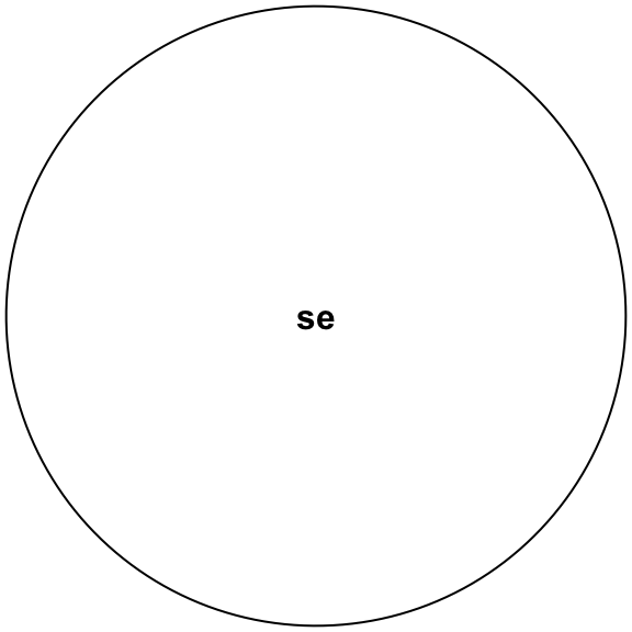
That spread — the differences from person to person — is the variability. We can visualize all that variability as a circle representing the total “pie” of variation in sleep efficiency (se):
Here’s the key question we’ll explore with our simulated data: Can we explain why people differ in their sleep efficiency?
- Is some of this variability predictable based on their alcohol consumption?
- How about their sleep hygiene?
- How about the combination of the two?
- How much of the variability can’t be explained by these factors?
Quantifying variability
Before we can partition this variability into explainable and unexplainable pieces, we need to measure it. We often use two related quantities to describe variability:
- Variance — the average squared distance from the mean:
\[ s^2 = \frac{1}{n - 1} \sum_{i=1}^{n} (y_i - \bar{y})^2 \]
- Standard deviation — the square root of variance (in original units1):
\[ s = \sqrt{\frac{1}{n - 1} \sum_{i=1}^{n} (y_i - \bar{y})^2} \]
Notice both formulas contain the Sum of Squares (SS) — that is, the total squared deviations:
\[ SS = \sum_{i=1}^{n} (y_i - \bar{y})^2 \]
This sum of squares for y (i.e., sleep efficiency) will be our starting point for understanding how regression works. Let’s compute it “by hand”, along with the variance and the standard deviation. Notice in the code that the sum of squares captures how far each individual’s sleep efficiency is from the overall sample mean, with each deviation squared and then summed.
Discussion Point
From Module 10 — you learned that through statistical models — we can split total variability into systematic (explained by predictors) and residual (unexplained by predictors) components.
outcome = systematic component + residual
As we begin to build our model to predict sleep efficiency — what would it mean if most of the variability ends up being residual? What would it mean if most is systematic? What makes a model ‘useful’ in terms of this partition?
Part II: Fitting a Simple Linear Regression
Now that we understand the total variability in sleep efficiency, let’s see if we can explain some of it using alcohol consumption.
Visualize the relationship
First, let’s look at the data. Create a scatter plot with alcohol consumption on the x-axis and sleep efficiency on the y-axis, including the best-fit line.
Discussion Point
Before fitting the regression and seeing the actual results, take a moment to examine the scatter plot carefully.
The slope: As alcohol consumption increases, does sleep efficiency appear to go up or down? By how much do you think sleep efficiency changes for each additional gram of alcohol consumed? Make a specific numerical guess.
The intercept: If someone consumed zero grams of alcohol, what sleep efficiency would you predict for them? Look at where the line would cross the y-axis and make your best estimate.
Strength of the relationship: How tightly are the points clustered around the best-fit line? Would you describe this as a strong relationship (points close to the line) or a weak relationship (points scattered far from the line)? What does this tell you about how well alcohol consumption predicts sleep efficiency?
Fit the model
Now let’s quantify this relationship precisely. Fit a simple linear regression model with sleep efficiency as the outcome and alcohol as the predictor. Call your model mod_1. Request the tidy() and glance() output from the broom package.
Discussion Point
Study the output carefully, and answer the following questions:
- Intercept: What sleep efficiency would we predict for someone who consumed 0 grams of alcohol?
- Slope (alcohol): For each additional gram of alcohol consumed, how does sleep efficiency change?
- \(R^2\): What proportion of the variability in sleep efficiency is explained by alcohol consumption?
- Sigma (\(\sigma\)): What’s the typical prediction error (in percentage points)?
- Were your initial predictions close?
- What story do these numbers tell about alcohol and sleep?
Peek inside: predictions and errors
Every regression model makes predictions. Use the augment() function to request the fitted values (i.e., the predictions) and residuals (i.e., the difference between the observed and fitted values).
Partitioning variability
Remember that circle representing all the variability in sleep efficiency? Regression lets us split that circle into multiple pieces.
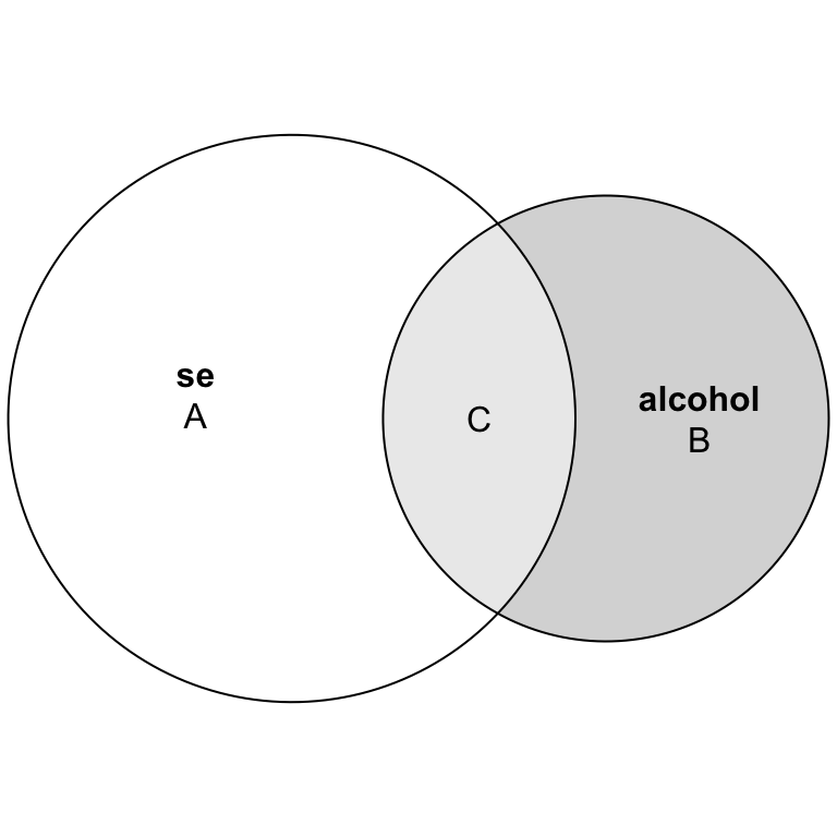
What each region in the Venn Diagram means:
- Region A: Variability in sleep efficiency that alcohol cannot explain (unexplained variance in se)
- Region B: Variability in alcohol consumption that doesn’t relate to sleep efficiency
- Region C: The overlap—variability in sleep efficiency that is predictable from alcohol (explained variance in se)
In regression terms (for the prediction of sleep efficiency):
- Region C = the systematic, predictable part (the variability in se that can be predicted by alcohol)
- Region A = the error, unpredictable part (the variability in se that cannot be predicted by alcohol)
This gives us R², the proportion of variance explained:
\[ R^2 = \frac{\text{explained variance}}{\text{total variance}} = \frac{\text{C}}{\text{A + C}} = 0.208 \]
Computing the partition by hand
Let’s verify this partition by calculating the pieces ourselves using the sum of squares:
Key Insights
- TSS = SSR + SSE: The total variability in sleep efficiency perfectly splits into explained (SSR) and unexplained parts (SSE)
- R² = SSR/TSS: This ratio tells us what fraction of the total variability we’ve explained
- R² = cor(y, ŷ)²: R² is literally the squared correlation between observed (y) and predicted (ŷ) values!
Think about it: An R² of 0.21 means alcohol consumption explains about 21% of why people differ in sleep efficiency. That leaves 79% unexplained — suggesting other factors matter too (like sleep hygiene!).
Discussion Point
Making sense of the sums of squares
After running the code above, examine the output carefully. You’ll see three key quantities: TSS, SSR, and SSE.
SSR (Sum of Squares Regression): This measures how far the predicted values (
.fitted) are from the overall mean. What does this distance represent? When predictions vary a lot from the mean, what does that tell us about how well alcohol explains differences in sleep efficiency?SSE (Sum of Squares Error): This measures how far the actual (i.e., observed) values are from the predicted values. These differences are the residuals. What kind of variability does this capture? If SSE were zero, what would that mean about our predictions?
The partition: Notice that SSR + SSE = TSS. What does this mathematical relationship tell us about how regression works? Which would we prefer to be larger — SSR or SSE — and why?
Connect to the Venn diagram: Looking back at the diagram with regions A and C, which sum of squares corresponds to which region? How does this help you understand what R² is actually measuring?
Understanding Sigma: The typical prediction error
We’ve measured how much variance we explained (R²), but how large are the actual prediction errors? That’s what sigma (\(\sigma\)) the residual standard deviation, also called the residual standard error, tells us.
\[ \sigma = \sqrt{\frac{1}{n - 2} \sum_{i=1}^{n} (y_i - \hat{y}_i)^2} \]
Compare to the standard deviation formula you saw earlier:
\[ s = \sqrt{\frac{1}{n - 1} \sum_{i=1}^{n} (y_i - \bar{y})^2} \]
Standard deviation of y, \(s\), measures spread around the overall mean
Sigma, \(\sigma\), measures spread around the regression line
Why n-2 for sigma? We estimated two parameters (intercept and slope), so we “lose” two degrees of freedom.
Click Run Code on the code chunk below to compute sigma “by hand” — then compare to the glance() output.
What sigma means
Here, sigma = 6.74, this means:
- On average, predictions are off by about 6.74 units (percentage points for sleep efficiency)
- This is the “typical” residual size
- It tells us the practical accuracy of our predictions
Visualize sigma
Let’s see what sigma looks like on our scatter plot:
Notice: Most points fall within one sigma of the regression line. This is what “typical error” means — it describes the general spread of residuals around our predictions.
Discussion Point
Comparing variability: We’ve reduced the typical prediction error from 7.56 (just guessing the mean — see the standard deviation of y calculated earlier) to 6.74 (using our model). That’s an 11% improvement: (7.56-6.74)/7.56. Does this seem like a meaningful reduction? What would need to happen for sigma to get much smaller?
Perfect predictions: Imagine sigma was 0. What would that mean about the relationship between alcohol and sleep efficiency? Why is this essentially impossible with real data?
Looking ahead: When we add sleep hygiene as a second predictor in our multiple regression, what do you predict will happen to sigma? Will it increase, decrease, or stay the same? Why?
Part III: Fitting a Multiple Linear Regression
We’ve seen that alcohol explains about 21% of the variability in sleep efficiency. But remember our study design — we also measured sleep hygiene. Can adding this second predictor help us explain more of the variation? Let’s find out!
To your SLR model, add sleep hygiene (shi) as an additional predictor. Call the model object mod_2. Request the tidy() and glance() output.
Discussion Point
The table below summarizes our two fitted models. Before moving on, compare Model 1 (the results from mod_1) and Model 2 (the results from mod_2). What changed? What stayed similar?
| Characteristic |
Model 1
|
Model 2
|
|---|---|---|
| Estimate | Estimate | |
| Intercept | 81.08 | 60.41 |
| Alcohol (grams) | -0.58 | -0.32 |
| Sleep Hygiene Index | 0.79 | |
| R² | 0.21 | 0.63 |
| Sigma | 6.74 | 4.64 |
Now, using the MLR estimates from tidy(), write out the full regression equation. Then test yourself: manually calculate the predicted sleep efficiency (ŷ) and residual for the first person in the dataset (their data is below):
Verify with augment
Use the augment() function to request the fitted values and residuals.
Important
Check the first case in the augmented data frame to ensure that you calculated their fitted value and residual correctly.
Interpret the estimates
Interpret the intercept and slope from the MLR. Using the estimate of the intercept and each slope from tidy(), jot down a few sentences to interpret the parameter estimates. Key phrase to remember: “holding other predictors constant” or “controlling for…”, or “comparing two people with the same score on all other predictors…”. Once you’re done, check your answer with the Interpretations tab.
Intercept (60.4): When both alcohol consumption and sleep hygiene are zero, we predict a sleep efficiency of 60.4%.
Alcohol slope (-0.32): For each additional gram of alcohol consumed, sleep efficiency decreases by 0.32 percentage points, holding sleep hygiene constant. This is the unique effect of alcohol after accounting for sleep hygiene.
Sleep hygiene slope (0.79): For each one-unit increase in sleep hygiene score, sleep efficiency increases by 0.79 percentage points, holding alcohol consumption constant. This is the unique effect of sleep hygiene after accounting for alcohol.
Visualizing Multiple Regression: The expanded Venn Diagram
With two predictors, our variance partition gets more interesting:
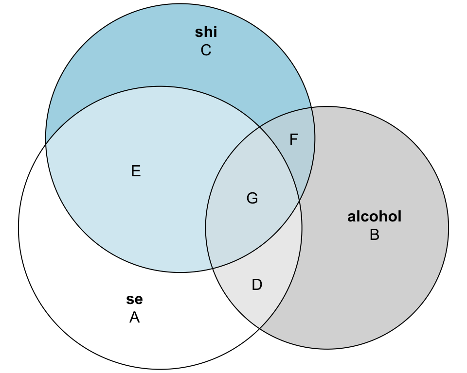
What each region of the sleep efficiency circle represents:
Region A: Variation in sleep efficiency that neither predictor explains (the remaining error)
Region D: Variation in sleep efficiency uniquely explained by alcohol (after accounting for sleep hygiene)
Region E: Variation in sleep efficiency uniquely explained by sleep hygiene (after accounting for alcohol)
Region G: Variation in sleep efficiency explained by both predictors (the shared/overlapping effect)
Thus, the variance in sleep efficiency that can be explained by the two predictors is represented by regions E, G and D. Thus, using this diagram, we can depict \(R^2\) for this model as:
\[ R^2 = \frac{\text{explained variance}}{\text{total variance}} = \frac{\text{D + E + G}}{\text{A + D + E + G}} = 0.627 \]
This tells us alcohol and sleep hygiene together explain 62.7% of the variation in sleep efficiency—much better than alcohol alone (21%)!
The Sigma Story: Tracking prediction accuracy
Let’s compare how our prediction accuracy has improved across models:
Find these values from your outputs and compare:
Standard deviation of se (from your earlier descriptive stats): ___
Sigma from mod_1 (alcohol only): ___
Sigma from mod_2 (alcohol + sleep hygiene): ___
What’s the pattern?
- The standard deviation of sleep efficiency represents prediction error if we ignore all predictors and just guess the mean
- Sigma from mod_1 shows prediction error after accounting for alcohol
- Sigma from mod_2 shows prediction error after accounting for both predictors
Each step reduces sigma — we’re getting better at predicting sleep efficiency! The progression from SD → sigma(mod_1) → sigma(mod_2) shows how adding meaningful predictors improves our model.
Discussion Point
The Changing Slope
The slope for alcohol changed from -0.58 (in the SLR) to -0.32 (in the MLR).
- Why did alcohol’s effect get smaller when we added sleep hygiene to the model?
- What does this tell us about the relationship between alcohol consumption and sleep hygiene in our sample?
Understanding the Venn Diagram
Look at the three-way Venn diagram with regions A through G.
- Region G represents variation explained by both predictors. What does it mean for two predictors to share explained variance? Why can’t we simply add up the individual R² values from two separate simple regressions?
- Region A represents unexplained variation. What factors might be contributing to this leftover variation in sleep efficiency?
The Prediction Accuracy Story
You should have three values: SD of sleep efficiency, sigma from mod_1, and sigma from mod_2.
- Calculate the percent reduction in prediction error from the SD to sigma (mod_1), and then from sigma(mod_1) to sigma (mod_2). Which step gave us the bigger improvement?
- If we could add one more predictor to further reduce sigma, what variable would you suggest measuring, and why?
Part IV: Understanding MLR through residuals (advanced bonus material)
Tip
Curious to explore further? The next section offers optional advanced material that builds on these concepts. Skip it if you’re ready to move on, or dive in if you want to deepen your understanding.
Here’s a mind-bending insight: The slope for alcohol in a MLR model can be recovered by working with residuals. This exercise reveals how multiple regression isolates the unique relationship between variables after “controlling for” others.
Step 1: Create the residuals
Our primary interest is understanding the relationship between alcohol consumption (alcohol) and sleep efficiency (se), while controlling for sleep hygiene (shi).
Our first step is to create the needed residuals and store them in a data frame called df_work.
Step 2: The partial relationship (residuals-on-residuals)
Now regress the y-residuals on the x-residuals. This gives us the partial regression coefficient for alcohol — and it will be identical to the alcohol coefficient from the full multiple regression model: lm(se ~ shi + alcohol).
Note
The double brackets [[ ]] are used here to tell R which coefficient to pull out of the regression model results. For example, coef(resid_model)[["x_resids"]] means “from the list of coefficients in resid_model, give me just the one named x_resids.” Likewise, coef(mod_both)[["alcohol"]] pulls out the alcohol slope from the multiple regression model. The point of this is just to create a little summary table.
They match. Partial regression (controlling for sleep hygiene) is the same as the MLR slope for alcohol.
The key idea: by using only the residuals, we are isolating the part of alcohol and sleep efficiency that is not explained by sleep hygiene, and then asking how those two “cleaned-up” variables relate to each other. The slope from this regression is the same as the slope for alcohol in the full MLR model. (Note: If you were to correlate these residuals instead of regressing them, you’d get the partial correlation — we’ll explore that distinction in Step 5.)
Step 3: The semi-partial correlation (unique contribution story)
The semi-partial correlation (called sr) is the correlation between original Y (se) and the residualized predictor (alcohol|shi). Note that this is not a regression slope — rather it is a correlation. Squaring the semi-partial correlation (sr²) gives the incremental R² that alcohol consumption adds beyond sleep hygiene in the MLR model.
Note
When you see code like df_work$x_resids, it simply means:
“From the data frame called df_work, take the column named x_resids.”
It’s a shorthand way in R to access a single variable inside a dataset. It works sort of like pull() from the tidyverse, but uses base R code.
Step 4: Verify sr² = ΔR²
As a sanity check, let’s compute R² for the model with sleep hygiene only, then for the model with sleep hygiene + alcohol. The difference in R² between these two models (ΔR²) should equal sr².
Insight: sr² = ΔR². Alcohol’s squared semi-partial correlation is exactly its unique contribution to variance explained in sleep efficiency beyond sleep hygiene. It asks: “How much will R² increase when we add our focal predictor (i.e., alcohol) to a model that already has the other predictor(s) (i.e., sleep hygiene).
Step 5: Partial vs. Semi-Partial correlations (clear comparison)
Up to now, we’ve focused on semi-partial correlation (sr), which helped us understand alcohol’s unique contribution to R². But there’s another closely related concept: the partial correlation (pr).
What’s the difference?
Both involve “controlling for” sleep hygiene, but they differ in how they do it:
- Partial correlation (pr): Correlation between y_resids (se|shi) and x_resids (alcohol|shi).
- “Remove sleep hygiene’s influence from both sides.”
- pr² = the proportion of sleep efficiency’s remaining variance (after controlling for sleep hygiene) that is explained by residualized alcohol (alcohol|shi). (Equivalently: R² from
lm(y_resids ~ x_resids).)
- Semi-partial correlation (sr): Correlation between se (original) and x_resids (alcohol|shi).
- “Remove sleep hygiene only from the predictor (alcohol).”
- sr² = ΔR², the extra variance in sleep efficiency explained by alcohol beyond what sleep hygiene explains. (Equivalently: R² from
(lm(se ~ shi + alcohol)) − R²(lm(se ~ shi))orcor(se, x_resids)^2.)
Let’s calculate both:
Intuition
- Partial (pr): “If I level the playing field by removing sleep hygiene’s influence from both alcohol and sleep efficiency, how strongly are they related?”
- Semi-partial (sr): “How much extra does alcohol add to explaining sleep efficiency, once sleep hygiene is already considered?”
Step 6: Map squared versions onto the Venn diagram
As a final step, let’s connect pr² and sr² to regions of our 3-way Venn diagram (A–G), continuing with our example where sleep hygiene is considered the “control” variable and alcohol is our “focal predictor.”
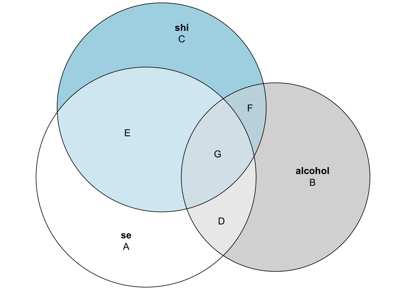
| Quantity | VennFormula |
|---|---|
| Partial correlation squared (pr²) | D / (A + D) |
| Semi-partial correlation squared (sr²) | D / (A + D + E + G) |
| ΔR² (add alcohol after shi) | D / (A + D + E + G) |
| R²(se ~ alcohol) | (D + G) / (A + D + E + G) |
| R²(se ~ shi) | (E + G) / (A + D + E + G) |
| R²(se ~ alcohol + shi) | (D + E + G) / (A + D + E + G) |
Putting it All Together
- Multiple regression partitions variance: Some variance is uniquely explained by each predictor, some is shared, and some remains unexplained
- Coefficients represent unique effects: Each slope tells you the effect of that predictor after accounting for all others
- R² increases with meaningful predictors: We went from 21% (alcohol alone) to 63% (alcohol + sleep hygiene)
- Sigma decreases with better predictions: Our typical prediction error dropped as we added sleep hygiene to the model
- Residuals reveal the mechanics: The residual regression shows why multiple regression coefficients differ from simple regression—they’re capturing unique, non-overlapping effects
Footnotes
Original units means the same units as your variable. Since sleep efficiency is measured in percentages, the standard deviation is in percentage points. Variance is in squared units (percentage points²), making it less intuitive to interpret.↩︎