A webR tutorial
Explore your own normal distribution
Explore Your Own Normal Distribution
Think of a continuous variable you’re interested in that might be normally distributed. Some examples:
SAT scores (mean ≈ 1050, sd ≈ 200)
Daily coffee consumption in ounces (mean ≈ 12, sd ≈ 4)
Reaction time in milliseconds (mean ≈ 250, sd ≈ 50)
Daily steps for college students (mean ≈ 8000, sd ≈ 2000)
Hours of sleep per night (mean ≈ 7.5, sd ≈ 1.2)
Modify the code below to explore your variable of interest. Click Run Code to see the result. Then use the prompts below the graph for further exploration/consideration.
Explore and consider
1) Translate vs. spread
Hold
my_sdfixed; changemy_mean.
→ Notice the curve shifts left/right but doesn’t change shape.Hold
my_meanfixed; changemy_sd.
→ Biggersd= wider & lower peak (area stays 1). Smallersd= narrow & tall.
2) Middle mass (area = probability)
Compare the printed “middle 95%” interval to the plot.
→ Is it symmetric around the mean? (It should be ~mean ± 1.96*sd.)Try
sdvalues that make the 95% range unrealistic for your variable — what does that tell you about a reasonablesd?
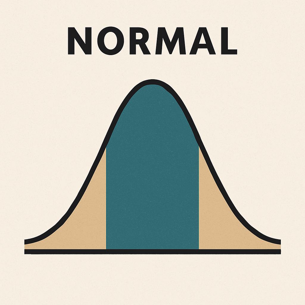
3) The 68–95–99.7 rule
Estimate by eye where
mean ± sd,mean ± 2*sd,mean ± 3*sdfall.How much of the curve seems to lie within each band? (≈ 68%, 95%, 99.7%.)
4) Percentiles & cutoffs (quantiles)
Find the value for the top 10%:
qnorm(p = 0.90, mean = my_mean, sd = my_sd).Find the median and quartiles:
qnorm(p = c(0.25, 0.5, 0.75), mean = my_mean, sd = my_sd).
5) Tail probabilities (single-sided & two-sided)
“What’s the chance a draw is above X?” →
1 - pnorm(q = X, mean = my_mean, sd = my_sd).“Between A and B?” →
pnorm(q = B, mean = my_mean, sd = my_sd) - pnorm(q = A, mean = my_mean, sd = my_sd).
6) Plausible domain
- If your variable can’t be negative (e.g., hours, steps), does your chosen
sdput non-trivial mass below 0?
→ If yes, consider a smallersdor note that a normal model may be imperfect at the lower tail.