A webR tutorial
NHST Exploration: Bootstrap and Parametric Approaches to a One-Sample t-test

The scenario
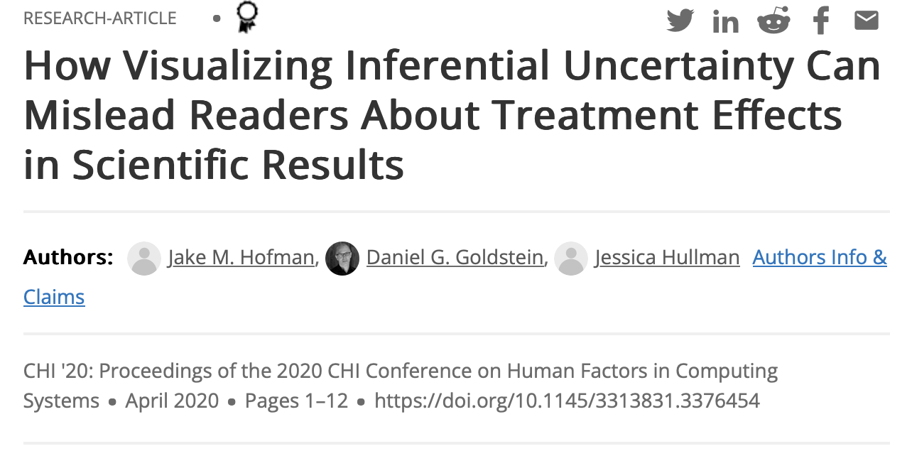
In this activity, we will work with data from this study conducted by Drs. Jake Hofman, Daniel Goldstein & Jessica Hullman. In Module 16, you studied data from their Experiment 1. Here, we’ll use data from Experiment 2.

Participants imagined competing in a boulder-sliding game against an equally skilled opponent named Blorg. They could rent a “special boulder” — a possible upgrade. Participants viewed one of four uncertainty visualizations about the special boulder and then reported their perceived probability of winning with it (our outcome: superiority_special — which ranges between 0 and 1).
Additionally, participants were randomly assigned to see either a small effect (probability of winning with the special boulder = 0.57, where 0.5 indicates even odds) or a large effect (probability of winning with the special boulder = 0.76). In this activity, we’ll focus on the participants who were randomly assigned to see visualizations depicting a large effect size.
Import the data
Click Run Code to import and prepare the data.
Visualize all conditions
This plot shows each visualization condition’s mean perceived win probability with a 95% CI, and the actual superiority (0.76) as a reference line.
Compare each condition’s CI to 0.76. If 0.76 is outside a CI, that group’s average perception likely differs from reality.
Choose your settings
Pick a condition, a significance level (α), and the number of resamples for the simulation.
Set up the selected condition
This extracts your chosen condition and prints the sample size and mean.
Simulate the null & compute a simulation-based p-value
We use the bootstrap to estimate sampling variability and then shift the bootstrap distribution so it is centered at μ₀ (the null). Then we count how often simulated means are as extreme or more extreme than the observed mean.
Visualize extreme samples
Why both tails? Our alternative is two-sided.
How bounds were set? Lower = μ₀ − |x̄ − μ₀|; Upper = μ₀ + |x̄ − μ₀|.
Parametric one-sample t-test (verification)
Now test the same hypothesis with a one-sample t-test using t_test() from the infer package. We then extract the t-statistic, degrees of freedom, and p-value, and make a decision at your chosen α.
Friendly decision table
Interpretation: Both approaches ask the same question in different ways. They should generally agree for the same α.
Visual: critical regions for your α
This plot shades the rejection regions of the Student’s t-distribution and marks the observed t-statistic from your selected condition.
Want to explore more?
- Try changing α to 0.10 or 0.01. How does the decision change?
- Increase reps (e.g., 10,000). Does the simulation p-value stabilize near the parametric p-value?
- Switch condition (e.g.,
"CI"or"HOPS"). Does perceived win probability tend to over- or under-estimate reality? - Choose a different null hypothesis value (i.e., mu0).