A webR tutorial
MLR with Uncorrelated Predictors
Background Information
From Observation to Experimentation
In the previous WebR activity, we explored an observational study where we measured people’s naturally occurring alcohol consumption and sleep hygiene habits. The reality of that data reflected real-world patterns: people who drank more alcohol also tended to have worse sleep hygiene. These variables were correlated, creating that overlapping Region G in our Venn diagram.
This correlation made interpretation tricky. When alcohol’s effect shrank from -0.58 to -0.32 after adding sleep hygiene to the model, we had to carefully disentangle which variable was doing what. The predictors were competing for credit in explaining sleep efficiency.
Why run an experiment?
But what if we could manipulate these variables instead of just observing them?
An experiment, with systematic assignment, can break the correlation. In this setting, someone with excellent sleep hygiene is just as likely to be assigned 0g of alcohol as 40g. The natural tendency for poor sleep hygiene and high alcohol consumption to co-occur can be eliminated by design.
Study Overview
To determine if alcohol consumption and sleep hygiene are predictive of sleep efficiency, you designed a randomized trial involving a diverse group of adults from Colorado. The study aims to provide insights into how these factors individually and collectively are associated with sleep quality.
Study Design
Type: Experimental study with a stratified random assignment
Population: Adults aged 21-65 years, selected from a state-level public health database focusing on sleep patterns among Colorado residents
Sample Size: 225 participants
Stratification and Systematic Assignment
Sleep Hygiene Blocking: Participants were first categorized into five groups based on their Sleep Hygiene Index (SHI) scores: 0 (poor hygiene), 10, 20, 30, and 40 (excellent hygiene). These groups served as blocking factors.
Alcohol Consumption Assignment: Within each SHI block, participants were randomly assigned to one of nine alcohol consumption levels: 0g, 5g, 10g, 15g, 20g, 25g, 30g, 35g, or 40g. Each of the 45 possible (SHI × alcohol) combinations was filled with an equal number of participants, creating a balanced factorial design.
The Key Feature: Orthogonal Predictors
This blocked random assignment produces orthogonal (uncorrelated) predictors. Unlike the observational study—where people with poor sleep hygiene tended to drink more alcohol—this design ensures that alcohol consumption is distributed identically across all SHI levels. A participant with excellent sleep hygiene (SHI = 40) is just as likely to be assigned 0g of alcohol as a participant with poor hygiene (SHI = 0).
What orthogonality means: The correlation between alcohol and sleep hygiene is exactly zero (r = 0) in expectation. Knowing someone’s alcohol assignment provides no information about their SHI group, and vice versa. This orthogonality eliminates the overlap (Region G) we saw in the MLR Venn diagram from the observational study, allowing us to cleanly separate each predictor’s unique contribution to explaining sleep efficiency.
Protocol
Each participant attended one evening study session. They were provided with their assigned amount of alcohol in a standardized beverage, ensuring consistency across all participants. Participants consumed the beverage between 6:00 and 9:00 pm, then wore validated sleep trackers overnight to measure sleep efficiency.
Simulate Data
Press Run Code on the code chunk below to create the simulated data frame (called data_uncorrelated) for this activity.
The variable called se represents sleep efficiency, which is the percentage of time in bed spent actually sleeping. For example, if an individual spends 8 hours in bed but only sleeps 6 hours, their sleep efficiency is 75%.
The variable called alcohol represents the grams of alcohol consumed.
The variable called shi represents the individual’s Sleep Hygiene Index (a higher value denotes better sleep hygiene).
Importantly, in this version of the study, because all combinations of sleep hygiene and alcohol use are systematically paired and replicated, the two predictors (sleep hygiene and alcohol) are completely uncorrelated by design.
You don’t need to understand how this simulation is working, but here’s some documentation in case you are interested. This code defines five levels of the Sleep Hygiene Index (SHI) — 0, 10, 20, 30, and 40 — to represent different levels of sleep hygiene practices among participants. It also specifies nine levels of alcohol consumption, ranging from 0 to 40 grams in increments of 5 grams. The code creates all possible combinations of SHI levels and alcohol consumption levels (using the expand_grid() function), resulting in a comprehensive grid of participant groups. Each combination is replicated five times to simulate multiple participants with the same SHI and alcohol consumption levels. This full factorial design ensures that the predictors (SHI and alcohol consumption) are uncorrelated by design. Finally, the code calculates the sleep efficiency for each simulated participant using a formula that includes a baseline value of 60, adds the product of 0.6 and the SHI score (implying that higher SHI scores increase sleep efficiency), subtracts the product of 0.4 and the alcohol consumption level (indicating that higher alcohol consumption decreases sleep efficiency), and adds a random error term drawn from a normal distribution with a mean of 0 and a standard deviation of 5.75 to mimic natural variability in sleep efficiency.
Descriptive statistics
In the code chunk below, use the skim() function from the skimr package to request descriptive statistics.
Take a look at the output to familiarize yourself with the variable distributions.
Fit a simple linear regression
Fit a simple linear regression model to quantify the relationship between alcohol (predictor) and sleep efficiency (outcome). That is, regress se on alcohol. Call your model object mod_1. Request the tidy() and glance() output from the broom() package.
Add sleep hygiene as a covariate
Now, to your SLR model, add sleep hygiene (shi) as an additional predictor. Call the model object mod_2. Request the tidy() and glance() output.
Discussion Point
Study the two outputs. What do you notice about how the estimate for the slope of alcohol has changed once sleep hygiene is added to the model? How does this differ from the changing effect of alcohol in the observational study that we examined in the prior WebR activity where alcohol and sleep hygiene were correlated?
The model as a Venn diagram
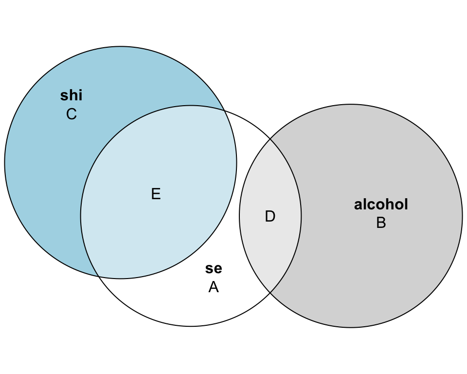
Now, to help further solidify your intuition, please study the Venn diagram below which depicts the uncorrelated predictors example from this activity.
Discussion Point
With your neighbor, use the Venn diagram above to define \(R^2\) using the lettered areas. How does this differ from the case where the predictors were correlated? Examine the \(R^2\) from the glance() output to quantify the variability in sleep efficiency that can be explained by alcohol and sleep hygiene.
Revisiting partial & semi-partial correlations with orthogonal predictors (advanced bonus material)
Tip
Curious to explore further? The next section offers optional advanced material that builds on these concepts. Skip it if you’re ready to move on, or dive in if you want to deepen your understanding.
In this experimental setup, alcohol and sleep hygiene (shi) are designed to be uncorrelated. That makes the relationships especially clean. Below, we will compute the partial and semi-partial correlations for alcohol and compare them to model-based quantities you fit earlier in the activity (mod_1: se ~ alcohol, mod_2: se ~ alcohol + shi).
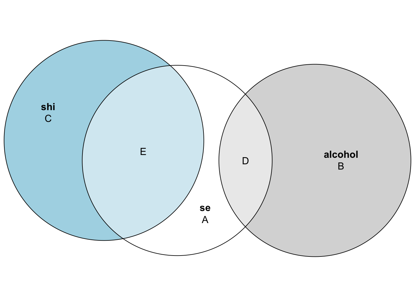
Mapping quantities to the Venn diagram
Now let’s connect pr² and sr² to the regions of our 3-way Venn diagram (A–G), using sleep hygiene as our control variable. The table below shows these relationships for both correlated and orthogonal predictors—notice how the formulas simplify dramatically when G disappears in the orthogonal case.
| Quantity | VennFormula | VennFormulaOrthogonal |
|---|---|---|
| Partial correlation squared (pr²) | D / (A + D) | D / (A + D) |
| Semi-partial correlation squared (sr²) | D / (A + D + E + G) | D / (A + D + E) |
| ΔR² (add alcohol after shi) | D / (A + D + E + G) | D / (A + D + E) |
| R²(se ~ alcohol) | (D + G) / (A + D + E + G) | D / (A + D + E) |
| R²(se ~ shi) | (E + G) / (A + D + E + G) | E / (A + D + E) |
| R²(se ~ alcohol + shi) | (D + E + G) / (A + D + E + G) | (D + E) / (A + D + E) |
The key insight shown here:
When G = 0:
sr² = ΔR² = R²(simple regression with alcohol alone): They all equal D / (A + D + E)
R²(alcohol + shi) = R²(alcohol) + R²(shi): The R² values are additive: D/(A+D+E) + E/(A+D+E) = (D+E)/(A+D+E)
This table demonstrates why orthogonal predictors make interpretation so clean: the unique contribution equals the total contribution for each predictor, and you can simply add up individual R² values to get the multiple R²!