A webR tutorial
Bayes’ Theorem and False Positives for a Rare Disease

Let’s imagine that a rare disease affects 1 in 1,000 people in the population. Fortunately, there is a highly accurate test for this disease. If an individual has the disease, the test correctly identifies it 99% of the time, meaning the test has a sensitivity (true positive rate) of 99%. However, the test also produces some false positives. Specifically, about 2% of people who do not have the disease will test positive.
You’ve just received a positive test result for the disease. Using the knowledge from Module 5 on the Basic Rules of Probability, you start calculating the likelihood that you actually have this rare disease.
First, you collate the information that you have available:
There are two pertinent events:
- Event DISEASE: You have the disease (and, given the information provided above, you know the \(P(\text{DISEASE}) = \frac{1}{1000} = 0.001\)).
- Event POSITIVE: You test positive for the disease.
You also know some information about the test’s effectiveness:
- The sensitivity of the test (also called the true positive rate) is \(0.99\), which means \(P(\text{POSITIVE} \mid \text{DISEASE}) = 0.99\).
- The false positive rate is \(0.02\) (2% of people who don’t have the disease will test positive). This means that the specificity of the test, which is the true negative rate, is \(1 - 0.02 = 0.98\).
You want to know: “What is the probability that I have the disease given that I tested positive?” This is a very important question to ask because the treatment for this very rare disease is extremely invasive and shockingly expensive.
To answer this question, you create a contingency table to divide the possibilities of your scenario into four mutually exclusive events. You outline the table below. This is also printed on the backside of your worksheet from lecture if you want to have a paper copy to work with.
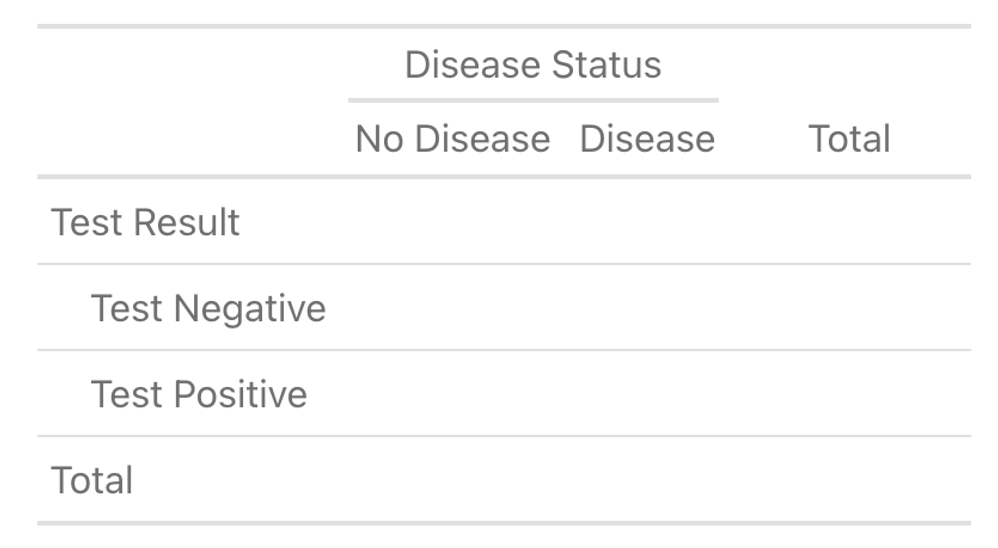
Using the constructed table, please fill in the quantities listed below. For example, the cell at the intersection of ‘Test Negative’ and ‘No Disease’ represents the probability of both testing negative and not having the disease. So, in this cell you’d write: \(P(\text{POSITIVE}^c \cap \text{DISEASE}^c)\).
Joint Probabilities
Probability of testing negative and not having the disease (True Negative): \(P(\text{POSITIVE}^c \cap \text{DISEASE}^c)\)
Probability of testing negative and having the disease (False Negative): \(P(\text{POSITIVE}^c \cap \text{DISEASE})\)
Probability of testing positive and not having the disease (False Positive): \(P(\text{POSITIVE} \cap \text{DISEASE}^c)\)
Probability of testing positive and having the disease (True Positive): \(P(\text{POSITIVE} \cap \text{DISEASE})\)
Marginal Probabilities
Probability of testing negative: \(P(\text{POSITIVE}^c)\)
Probability of testing positive: \(P(\text{POSITIVE})\)
Probability of not having the disease: \(P(\text{DISEASE}^c)\)
Probability of having the disease: \(P(\text{DISEASE})\)
Once you’ve done this on your own, check the completed contingency table below to be sure you have the right result:
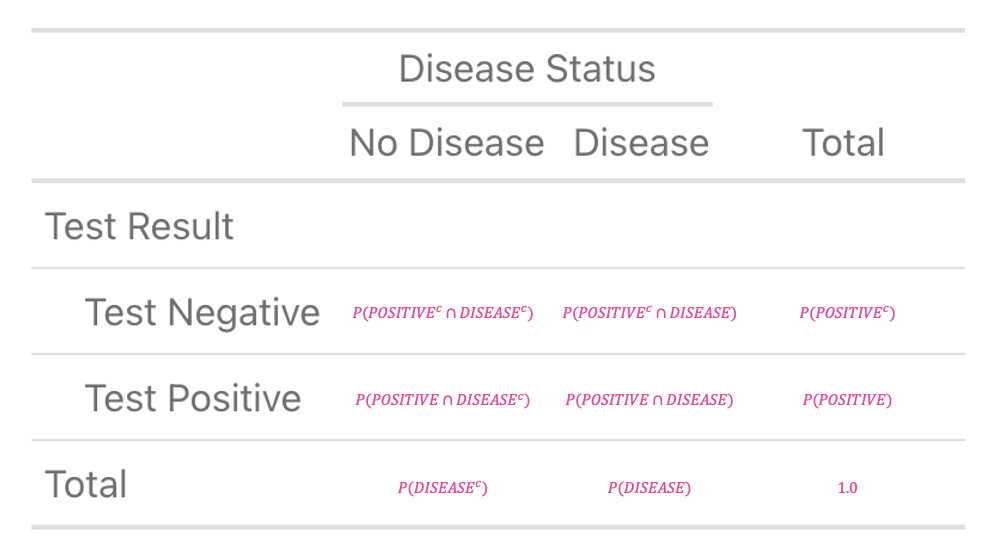
Now, that you have the table structure, you begin to fill in the known quantities.
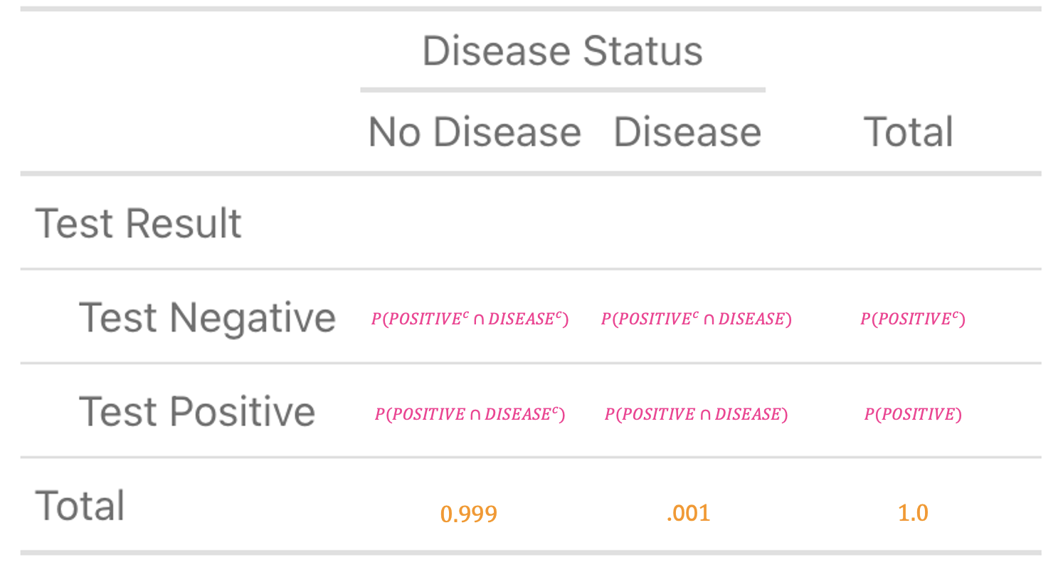
You start with the row margins, which refers to the probability of not having the disease \(P(\text{DISEASE}^c)\) and the probability of having the disease \(P(\text{DISEASE})\). You were told that the probability of disease is \(0.001\). Therefore the probability of not having the disease is \(1 - 0.001 = 0.999\) (this is the Law of Total Probability).
Plugging in these values, your table should look like this:
Next, you solve for \(P(\text{POSITIVE} \cap \text{DISEASE})\). We learned in Module 5 that when the events are related, we can apply the following formula to solve for the joint probability (e.g., testing positive and having the disease).
\[ P(\text{POSITIVE} \cap \text{DISEASE}) = P(\text{POSITIVE} \mid \text{DISEASE}) \times P(\text{DISEASE}) \]
The first value, \(P(\text{POSITIVE} \mid \text{DISEASE})\), is the tests’ sensitivity. We were given this value (\(0.99\)). The second value is the disease prevalence in the population, which we were also given (\(0.001\)). Thus, we can solve for \(P(\text{POSITIVE} \cap \text{DISEASE})\) as follows:
\[ P(\text{POSITIVE} \cap \text{DISEASE}) = P(\text{POSITIVE} \mid \text{DISEASE}) \times P(DISEASE) = 0.99 \times 0.001 = 0.00099 \]
Now, you move to solve for \(P(\text{POSITIVE} \cap \text{DISEASE}^c)\). This is also a joint probability, and can be calculated using the following formula:
\[ P(\text{POSITIVE} \cap \text{DISEASE}^c) = P(\text{POSITIVE} \mid \text{DISEASE}^c) \times P(\text{DISEASE}^c) \]
The quantities to the right of the equals sign were given to you, so you can plug in and solve as follows:
\[ P(\text{POSITIVE} \cap \text{DISEASE}^c) = P(\text{POSITIVE} \mid \text{DISEASE}^c) \times P(\text{DISEASE}^c) = 0.02 \times 0.999 = 0.01998 \]
Because you have now solved for both \(P(\text{POSITIVE} \cap \text{DISEASE})\) and \(P(\text{POSITIVE} \cap \text{DISEASE}^c)\), you can sum these to solve for \(P(\text{POSITIVE})\) — which is \(0.00099 + 0.01998 = 0.02097\). Take a moment to plug these numbers into your table.
Verify that you’ve done this correctly with the table below:
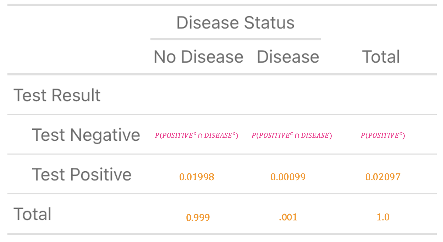
Now, you can find the remaining probabilities to complete your table by subtracting in the columns and adding across the remaining row. That is, \(0.999 - 0.01998 = 0.97902\). Likewise \(0.001 - 0.00099 = 0.00001\). Finally \(0.97902 + 0.00001 = 0.97903\). The completed table is below:
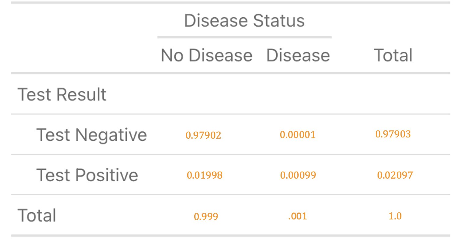
Hooray, the table is complete and you’re ready to answer the question: “What is the probability that I have the disease given that I tested positive?” This is a conditional probability \(P(\text{DISEASE} \mid \text{POSITIVE})\), which can be calculated using the row labeled ‘Test Positive’.
The formula is:
\[ P(\text{DISEASE} \mid \text{POSITIVE}) = \frac{P(\text{DISEASE} \cap \text{POSITIVE})}{P(\text{POSITIVE})} = \frac{0.00099}{0.02097} = 0.047 \]
So, the chance you have the disease given a positive test result is approximately 4.7%.
Recall from Module 5 that we called this conditional probability that you just calculated the Positive Predictive Value (PPV). The take home message here is, even though the test for the disease is highly accurate, less then 5% of people who test positive will actually have the disease. Therefore, before you spend a lot of money to treat the disease, you should probably consider additional assessments.
Using Bayes’ Theorem, you could have avoided all of these computations (though, of course, they’re good practice). That is, Bayes’ Theorem can be used to calculate the Positive Predictive Value (PPV) as follows:
\[ PPV = P(\text{DISEASE} \mid \text{POSITIVE}) = \frac{P(\text{DISEASE} \cap \text{POSITIVE})}{P(\text{POSITIVE})} \]
This can be expanded to:
\[ PPV = \frac{P(\text{POSITIVE} \mid \text{DISEASE}) \times P(\text{DISEASE})}{P(\text{POSITIVE} \mid \text{DISEASE}) \times P(\text{DISEASE}) + P(\text{POSITIVE} \mid \text{DISEASE}^c) \times P(\text{DISEASE}^c)} \]
Where:
- \(P(\text{POSITIVE} \mid \text{DISEASE})\) is the sensitivity of the test.
- \(P(\text{DISEASE})\) is the prior probability of having the disease (prevalence).
- \(P(\text{POSITIVE} \mid \text{DISEASE}^c)\) is the probability of a false positive (1 - specificity).
- \(P(\text{DISEASE}^c)\) is the prior probability of not having the disease (1 - prevalence).
Plugging in the numbers we get:
\[ PPV = \frac{0.99 \times 0.001}{(0.99 \times 0.001) + (0.02 \times 0.999)} = 0.047 \]
Explore a bit more with a simulation
In diagnostic testing, the Positive Predictive Value (PPV) represents the probability that an individual actually has a disease given that they have tested positive for it. PPV is influenced by three main factors:
The sensitivity of the test (the true positive rate)
The specificity of the test (the true negative rate)
The prevalence of the disease (how common the disease is in the population).
Let’s explore how these factors change the PPV.
First, press Run Code on the code chunk below to create a function called calculate_ppv().
Now, let’s use the function to solve for the PPV. To begin let’s plug in the three needed parameters for the rare disease example we just completed.
Your Turn to Explore: Use the function to see how changes in prevalence, sensitivity, and specificity affect the PPV. Change these values in the code chunk below to explore.
Tips for Exploration:
Examples to Try:
Increase Prevalence: Start with a higher prevalence, such as
prevalence = 0.25, to see how it impacts the PPV.Change Sensitivity: Try adjusting the sensitivity. For instance, what happens if sensitivity drops to
0.90or increases to1.0?Change Specificity: Adjust the specificity, e.g., lowering it to
0.95or increasing it to0.99.
Observations to Make:
How does PPV change when the disease is more common?
How sensitive is the PPV to changes in specificity versus sensitivity?
Interesting Points to Ponder if Intrigued:
Effect of Prevalence: When the prevalence of a disease is low, even a test with high sensitivity and specificity can have a low PPV. This is because the number of false positives might outweigh the true positives. Conversely, with a high prevalence, the PPV tends to be higher because the proportion of true positives increases.
Balance Between Sensitivity and Specificity: High sensitivity ensures that most actual cases are detected (low false negative rate), but if specificity is not also high, there can be many false positives, leading to a lower PPV. This is particularly crucial in diseases with low prevalence, where the false positives can dominate.
Impact on Decision Making: A low PPV implies that many positive test results are actually false positives. This can have significant implications, such as unnecessary anxiety, further testing, and treatment. High PPV is desirable to ensure that a positive test result is a strong indicator of the disease.
Clinical and Public Health Implications: Understanding these dynamics is essential for developing screening guidelines and determining which populations to screen. For instance, a test might be useful for a high-risk population (with higher prevalence) but not for the general population.
Credits
The example used in this tutorial comes from the wonderful book entitled “The Cartoon Guide to Statistics” by Larry Gonick and Woollcott Smith.