A webR tutorial
MLR with Correlated Predictors

Background information
Sleep is a vital component of overall health and well-being. Sleep efficiency (SE) — the percentage of time spent asleep while in bed — is a key indicator of sleep quality. Alcohol consumption is known to affect our sleep, potentially reducing sleep efficiency by disrupting normal sleep patterns. Conversely, the Sleep Hygiene Index (SHI) measures an individual’s engagement in behaviors that promote healthy sleep, such as maintaining a regular sleep schedule, creating a restful environment, and limiting exposure to screens before bedtime.
Study Overview
To determine if alcohol consumption and sleep hygiene are predictive of sleep efficiency, you designed a study involving a diverse group of adults from Colorado. The study aims to provide insights into how these factors individually and collectively are associated with sleep quality.
Study Design
Type: Observational study.
Population: Adults aged 21-65 years, selected from a state-level public health database focusing on sleep patterns among Colorado residents. The database consists of a representative sample of Colorado adults.
Sample Size: You randomly select 225 adults from the database and invite them to participate in the study.
Protocol: One evening study session was selected for each participant. On their selected day, the participant was provided with 40 grams of alcohol. The alcohol was presented in a standardized beverage, ensuring consistency across participants. Participants were instructed to consume as much or as little of the provided alcohol as they wished, but not to drink any other alcoholic beverages. They were instructed to drink the provided alcohol between the hours of 6 and 9 pm. They were informed that there was no expectation or requirement to consume the entire amount. The remaining alcohol was measured after the session to determine the exact intake. This approach allowed for precise quantification of individual alcohol consumption without influencing participants’ natural drinking behaviors. That night, sleep efficiency was measured using a wearable sleep tracker that recorded sleep patterns throughout the night. Devices were validated for accuracy and reliability in sleep studies.
Simulate data
Press Run Code on the code chunk below to create the simulated data frame for this activity. The produced data frame is called data_correlated.
The variable called se represents sleep efficiency, this is the outcome variable that we want to predict.
The variable called alcohol represents the grams of alcohol consumed.
The variable called shi represents the individual’s Sleep Hygiene Index score (a higher value denotes better sleep hygiene).
You don’t need to understand how this simulation is working, but here’s some documentation in case you are interested. This code generates a simulated dataset for a study exploring the relationships between sleep efficiency (se), Sleep Hygiene Index (shi), and alcohol consumption (alcohol) using the faux package. It begins by setting a random seed for reproducibility. Then, it defines the number of participants (225) and specifies the average values (means) and variability (standard deviations) for each variable. The code sets the desired correlations between the variables — specifically, a strong positive correlation between sleep efficiency and sleep hygiene (0.75), a moderate negative correlation between sleep efficiency and alcohol consumption (-0.4), and a small to moderate negative correlation between sleep hygiene and alcohol consumption (-0.3). Finally, it uses these parameters to generate the dataset, creating realistic data that reflects the specified relationships among the variables for further analysis. You’ll get a lot of opportunities to learn about simulating data for studying statistical principles in PSY653, for now, you don’t need to worry about the details of how simulation studies are set up.
Descriptive statistics
In the code chunk below, use the skim() function from the skimr package to request descriptive statistics.
Additionally, use the correlate() function from the corrr to request the correlation matrix.
Jot down a few sentences to describe the descriptive statistics as well as the correlation matrix.
Alcohol and sleep efficiency
Next, please create a scatter plot of alcohol (on the x-axis) and sleep efficiency (on the y-axis). Include the best fit line.
When plotting raw variables (e.g., alcohol consumption and sleep efficiency), the slope of the best-fit line (also known as the regression line) represents the magnitude of the effect of the predictor variable on the outcome variable. Specifically, it tells you how much the outcome variable is expected to change for a one-unit increase in the predictor variable. Can you guess what the intercept and slope are for this best fit line?
Fit a simple linear regression
Please fit a simple linear regression model to quantify the relationship between alcohol and sleep efficiency. Call your model object mod_1. Request the tidy() and glance() output from the broom() package.
Study the equation
Study the output. Identify the intercept and slope of the best fit line. Was your guess from the scatter plot close? Jot down a few sentences to describe these results. Then, compare notes with your neighbor.
Examine the fitted values and residuals
Please use the augment() function to request the fitted values and residuals.
Practice calculation of fitted values and residuals. Choose one observed case, using the fitted model, verify that you can recover the fitted value and residual.
Proportion of variance explained for the SLR
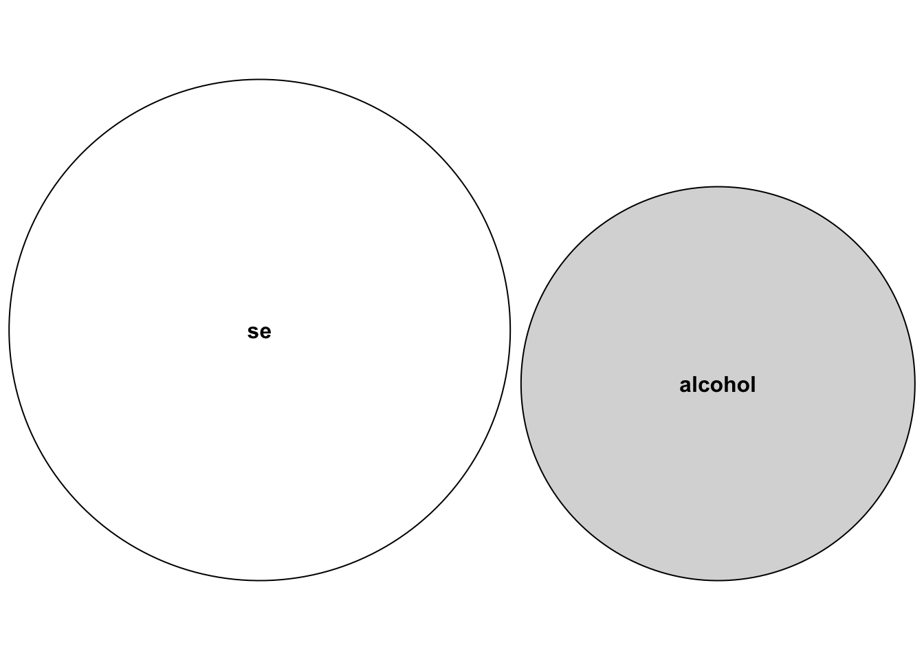
The diagram below depicts the variability in sleep efficiency (se) and alcohol as two separate circles.
Additionally, we can visualize the covariance between these two variables — this is depicted in the diagram below. I will label the three regions for clarity. Here, A represents the variability in sleep efficiency that is unrelated to alcohol, C represents the variability in alcohol that is unrelated to sleep efficiency. The area labeled C denotes the amount of variation in sleep efficiency that can be predicted by alcohol consumption.
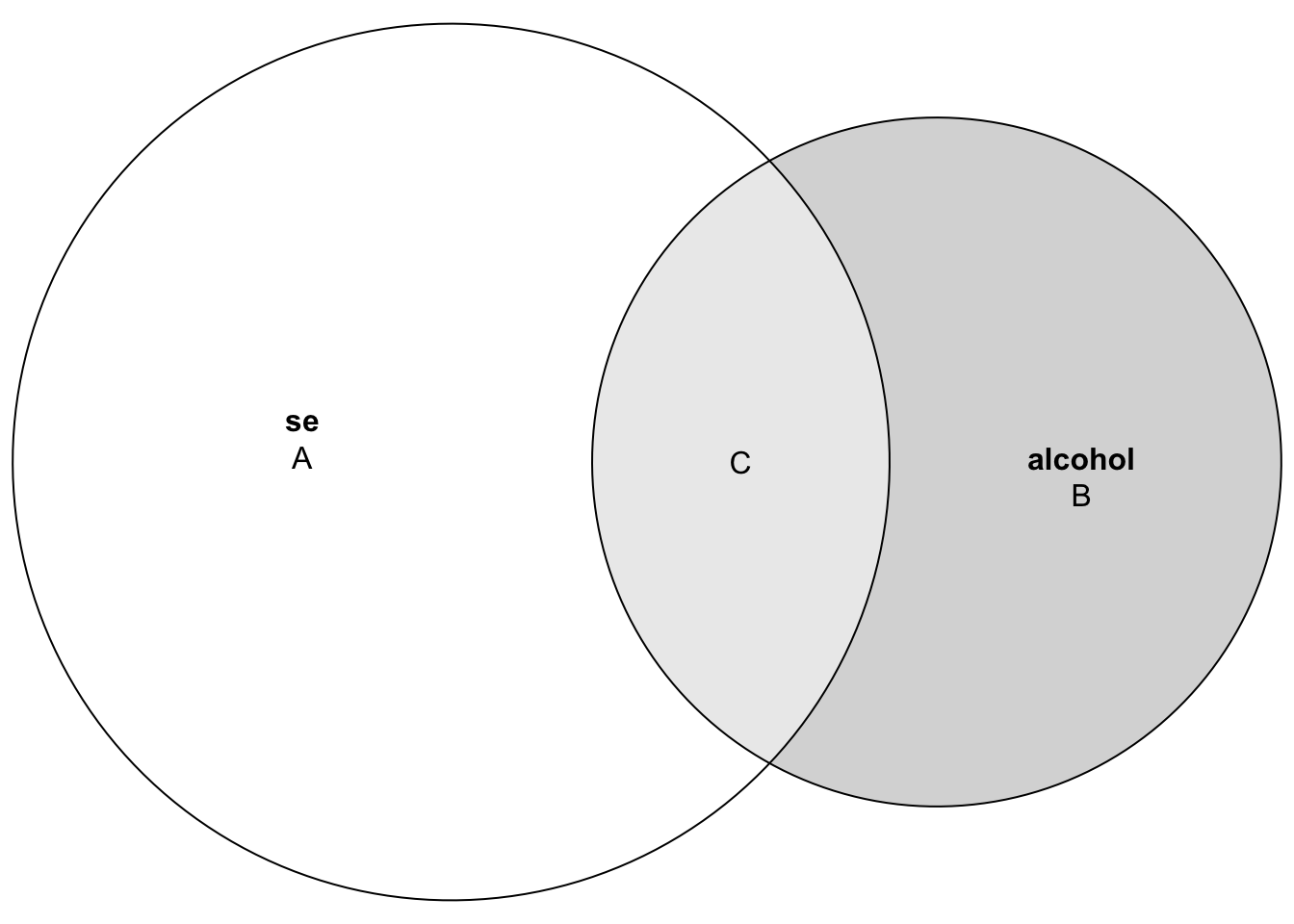
In thinking about our regression model — where the total variability in the outcome (sleep efficiency) can be partitioned into the part explained by the model (i.e., the systematic part), and the part unexplained by the model (i.e., the error) — area C depicts the systematic part and area A depicts the error.
\[ R^2 = \frac{\text{explained variance}}{\text{total variance}} = \frac{\text{C}}{\text{A + C}} = 0.208 \]
With this information in hand, go back to the glance() output from the model. Identify the \(R^2\). Compare the sigma to the standard deviation of the outcome (se) from the descriptive statistics output that you created earlier. How does the standard deviation compare to sigma? Verify that you can compute the same value for \(R^2\) using the standard deviation of sleep efficiency and sigma from the SLR — just as we did in the intro slide deck. Also notice that the correlation of se and alcohol from the correlation matrix computed earlier can be used to obtain \(R^2\), where the square of the correlation equals the \(R^2\). That is, in simple linear regression with a single predictor, the square of the correlation between the predictor (alcohol) and the outcome (se) is equal to \(R^2\). Jot down a few sentences to describe these results. Then, compare notes with your neighbor.
Fit a multiple linear regression
Now, to your SLR model, add sleep hygiene (shi) as an additional predictor. Call the model object mod_2. Request the tidy() and glance() output.
Study the estimates from the tidy() output. Write down the regression equation, then solve for the fitted score (y-hat) and the residual for the first case in the data frame:
Examine the fitted values and residuals
Please use the augment() function to request the fitted values and residuals.
Check the first case in the data frame to ensure that you calculated their fitted value and residual correctly.
Interpret the estimates
Interpret the intercept and slope. Using the estimate of the intercept and each slope from tidy(), jot down a few sentences to interpret the parameter estimates. Once you’re done, check your answer with the answer tab.
The intercept estimate of 60.4 indicates that, when both alcohol consumption and sleep hygiene (shi) are at zero, the predicted sleep efficiency is 60.4%. This serves as the baseline level of sleep efficiency when no alcohol is consumed and no sleep hygiene behaviors are reported.
The slope for alcohol is -0.318, meaning that for each additional unit of alcohol consumed, sleep efficiency decreases by 0.318 percentage points, holding sleep hygiene constant.
The slope for sleep hygiene (shi) is 0.791, suggesting that for each additional unit of sleep hygiene score, sleep efficiency increases by 0.791 percentage points, holding alcohol consumption constant.
Change in the effect of alcohol
Take a moment to compare how the effect of alcohol has changed from the SLR to the MLR. Jot down a few sentences to describe what you think that might mean?
Proportion of variance explained for the MLR
To further understand the MLR results, we can grow our Venn diagram to accommodate the additional predictor. This is displayed below.
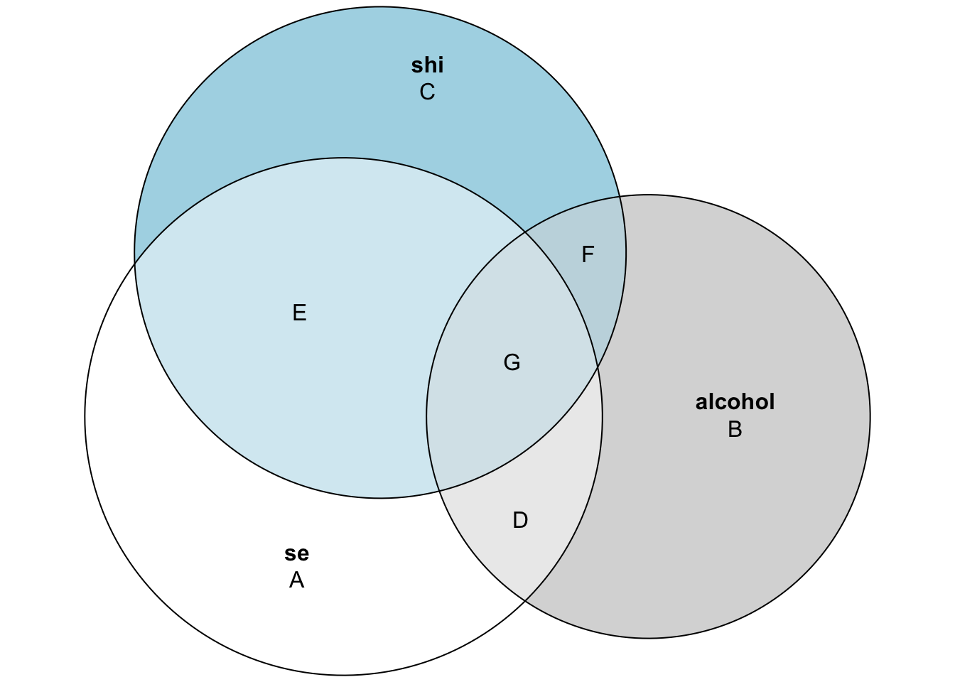
The individual circles for se, alcohol, and shi represent each variable’s total variance, while overlapping areas represent shared variance amongst the variables. From the diagram, we see that both alcohol and shi explain some of the variation in se — with shi explaining more of the variability than alcohol. Area D denotes the variation in se that can be uniquely predicted by alcohol, while area E represents the variation in se that can be uniquely predicted by sleep hygiene. The area labeled G is the part of the variation in se that can be predicted by both alcohol and sleep hygiene.
Thus, the variance in se that can be explained by the two predictors is represented by regions E, G and D. Thus, using this diagram, we can depict \(R^2\) for this model as:
\[ R^2 = \frac{\text{explained variance}}{\text{total variance}} = \frac{\text{D + E + G}}{\text{A + D + E + G}} = 0.627 \]
With this information in hand, go back to the glance() output from the MLR model. Identify the \(R^2\). Compare the sigma from the MLR model to the sigma from the SLR model and to the standard deviation of the outcome (se) from the descriptive statistics output that you created earlier. Write down and label all three. How does the standard deviation compare to sigma from the MLR? How does sigma from the SLR model compare to sigma from the MLR model? Jot down a few sentences to describe these results. Then, compare notes with your neighbor.
Recovering estimates via residuals
By studying the residuals, we can further understand the regression estimates.
In the code chunk below, notice first the provided code in which I regress se on shi. Then augment() is used to save the resulting residuals. To denote that these are the “y-variable” residuals (i.e., they result from regressing the outcome (y) on sleep hygiene), I’ve renamed them y_resids.
Underneath this code, add similar code to regress alcohol on shi and save the residuals. To denote that these are the “x-variable” residuals, rename them x_resids.
Now that we have both sets of residuals. We can combine them into a data frame. I’ve done this for you below. Now, using this new data frame, please regress the y_resids on the x_resids. Request the tidy() output. Study the output and determine where you’ve seen the regression estimate for the slope before.
Take a moment to think about the residuals resulting from the two models. What information does each contain? Why does regressing the y_resids on the x_resids return the regression coefficient for the effect of alcohol in the MLR? Jot down your answers, discuss with your neighbor, then we’ll discuss as a group.
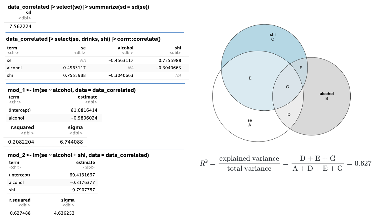
A summary for our discussion
’