A webR tutorial

Explore the probability distribution of baby weights

Introduction

The average newborn baby in the US weighs 3254.42 grams, standard deviation = 587.73. Baby weights are normally distributed in the population — therefore we can use the qnorm() and pnorm() functions in R to describe the distribution of baby weights.

Example 1

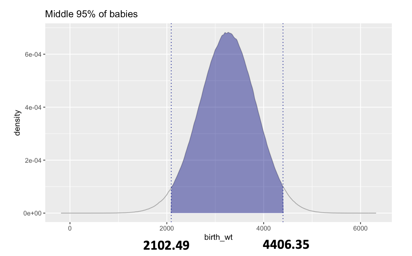
What range of birth weights will encompass the middle 95% of the distribution?

code

hint

For this, we need to find the 2.5th and 97.5th percentiles of the distribution. The qnorm() function in R will calculate these. Input the desired percentile first, then the mean and standard deviation for our normal distribution of baby weights.

solution

Answer: 95% of new born babies will weigh between 2102.49 grams and 4406.35 grams.

Example 2

Building on the solution to Example 1, convert the baby weight for the 2.5th percentile and the 97.5th percentile of the distribution to z-scores.

code

hint

Recall that a z-score is formed by subtracting the mean and dividing by the standard deviation. So for example, to compute the the z-score the for 2.5th percentile you can take:

low_z = (2102.49 - 3254.42)/587.73

solution

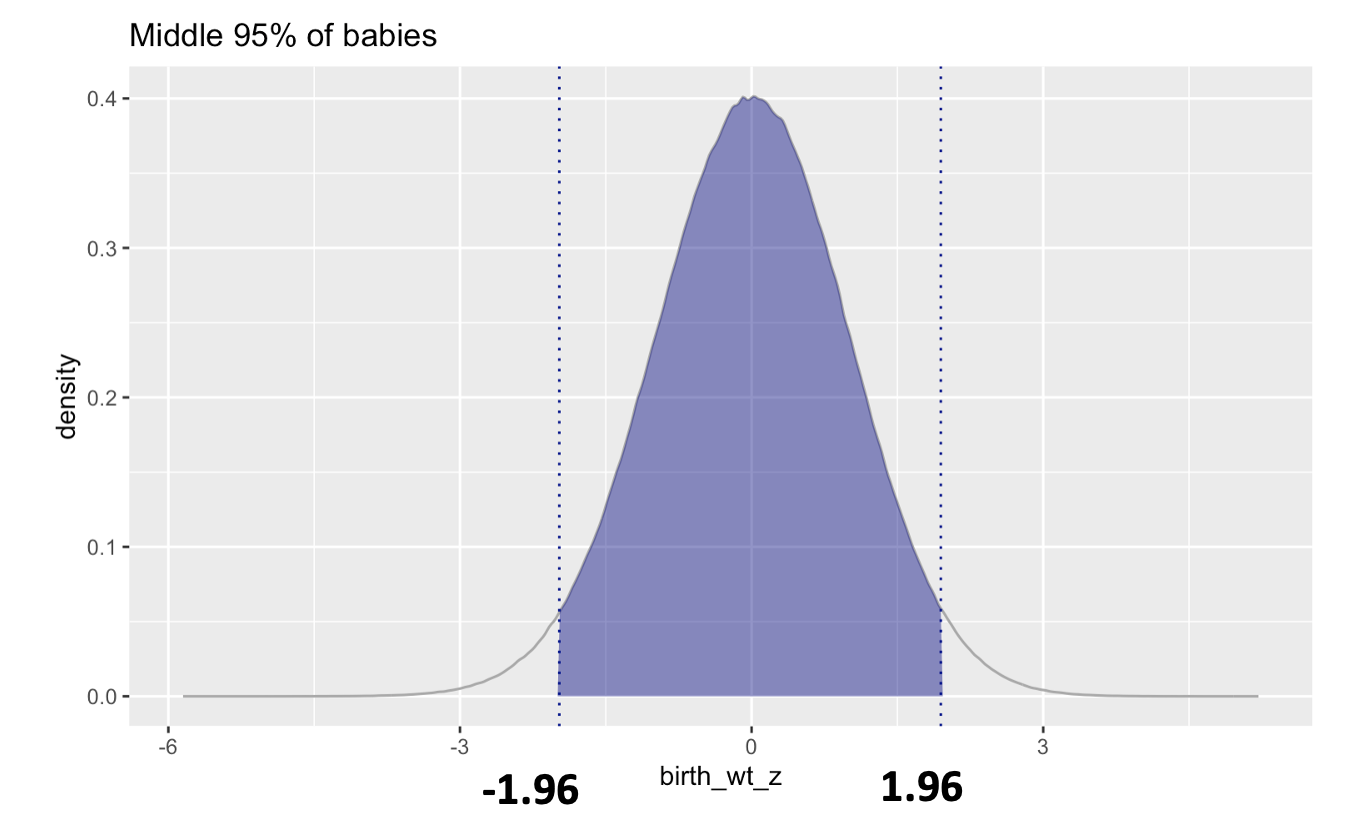
Answer: This tells us that if a baby is at the 2.5th percentile, their z-score is -1.96 (they weigh 1.96 standard deviations below the mean). If a baby is at the 97.5th percentile, their z-score is 1.96 (they weigh 1.96 standard deviations above the mean).

This graph shows the distribution of newborn baby weights in z-scores (birth_wt_z). Using the probability density function for this normal distribution — we estimate that 95% of the babies born will weigh within 1.96 standard deviations of the mean.

Example 3

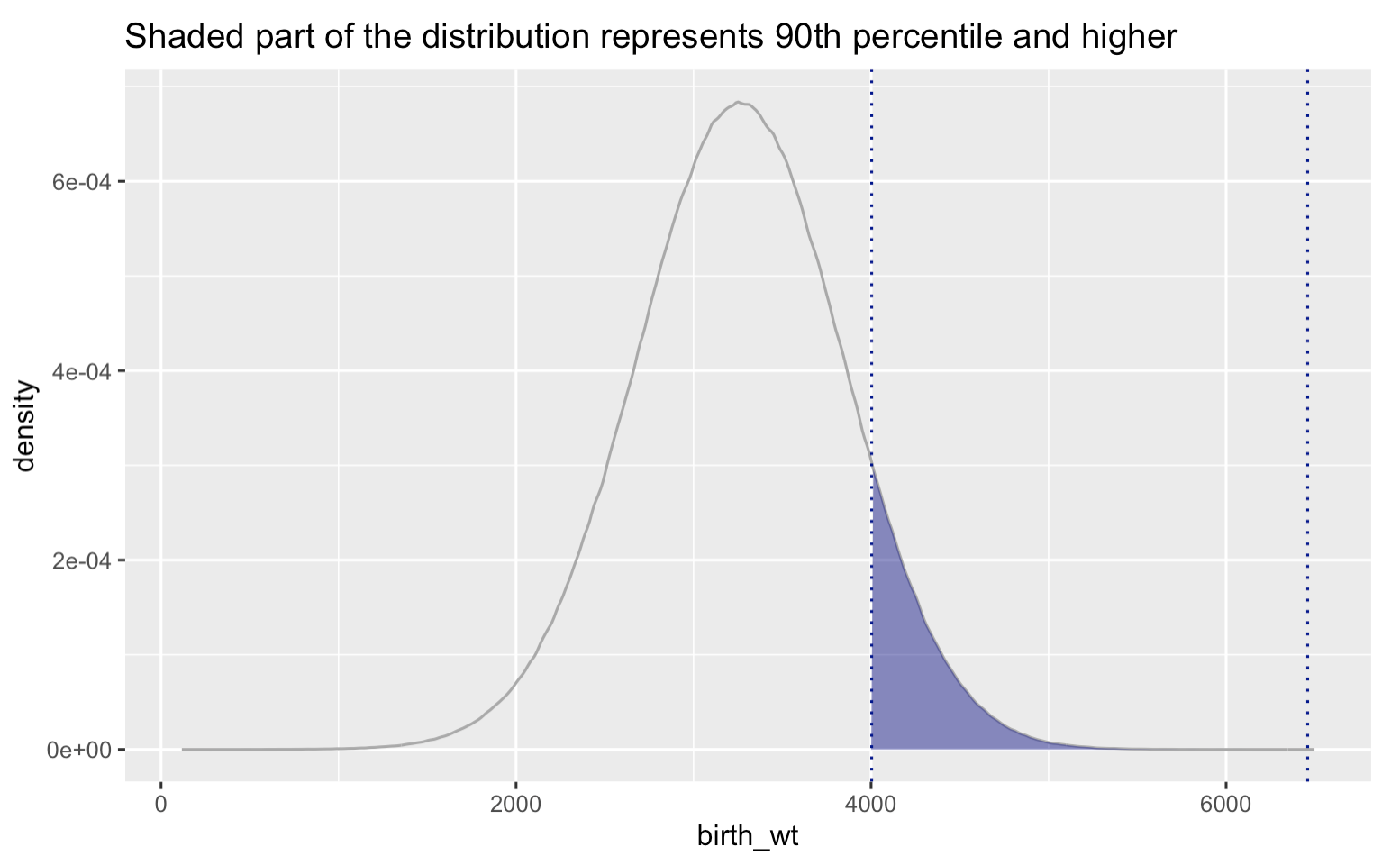
How much does a newborn need to weigh to be in the top 10% of the distribution?

code

hint

For this, we need to find the 90th percentile of the distribution. The qnorm() function in R will calculate this. Input the desired percentile first, then the mean and standard deviation for our normal distribution of baby weights.

solution

Answer: A baby needs to weigh at least 4007.63 grams to be in the top 10% for weight (i.e., the 90th percentile or higher).

Example 4

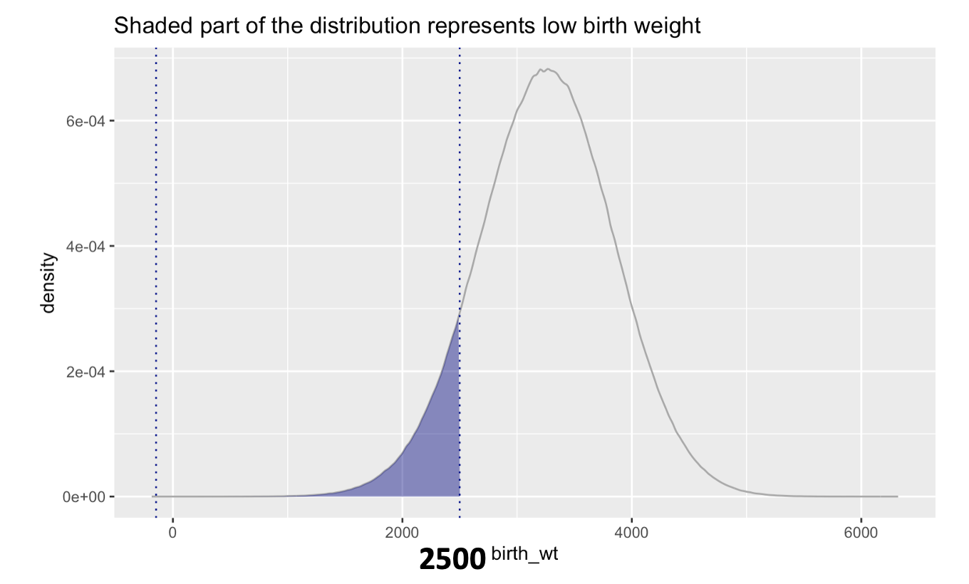
Low birth weight is a term used to describe babies who are born weighing less than 2500 grams (5 pounds, 8 ounces). What is the probability that a baby will be classified as low birth weight?

code

hint

For this example, we’re solving for a probability not a quantile — therefore, we use pnorm(). Enter the weight we want to solve for, and the mean and sd of our normal distribution.

solution

Answer: The probability that a baby will be classified as low birth weight (i.e., weigh 2500 grams or less) is about .10.

Example 5

Now, let’s solve for the complement of Example 4. What is the probability that a baby will be classified as having a normal birth weight (i.e., above 2500 grams)? Note that there is a condition called macrosomia, which refers to very large babies, typically those weighing more than 4000 or 4500 grams. However, for simplicity, we’ll ignore macrosomia here and consider all babies weighing at least 2500 grams as having a normal birth weight.

code

hint

To solve for our desired quantity, we just need to add an indication that we want the upper tail of the distribution. Recall that the default for pnorm() is lower.tail = TRUE.

solution

Answer: The probability that a baby will be classified as normal birth weight (i.e., weigh 2500 grams or more) is about .90.

Some commentary on the lower.tail argument

For those who might be curious, the lower.tail argument is available in both pnorm() and qnorm(), though it is typically more useful for pnorm() than for qnorm(), and here’s why:

• pnorm() returns the cumulative probability for a given value (i.e., the area under the curve to the left of that value). By default, it calculates the probability from the lower tail (left side), but setting lower.tail = FALSE allows you to compute the probability from the upper tail (right side). This can be very useful when you want to calculate the probability of being greater than a given value rather than less than (as we’ve practiced a few times in the Module handout and the lecture slides).

• qnorm(), on the other hand, calculates the quantile for a given probability. Since you’re often interested in percentiles (which are usually calculated from the lower tail), lower.tail is less frequently adjusted here. However, you can still use lower.tail = FALSE to find the complementary quantile from the upper tail, which can be helpful in some cases (e.g., finding the value that corresponds to the top 10% rather than the bottom 90%).

For example, the code below provides two different methods of finding the same quantile: